D Estimating Age of Acquisition
It is frequently useful to have an estimate of the age at which children produce a particular word with a probability greater than some threshold; these are commonly referred to as the word’s age of acquisition (AoA; Goodman, Dale, and Li 2008). In this Appendix, we compare methods for estimating age of acquisition, using the English Words & Sentences data as a case study.
The simplest and most obvious measure is to use the empirically-determined first month at which the proportion producing a word exceeds the threshold. We will use 50% of children producing as our threshold in all subsequent discussion, following previous literature (Goodman, Dale, and Li 2008). This approach is simple, but results in the exclusion of a large number of words. Of the total, 11% do not reach 50% production by the ceiling of the form and must be discarded. Further, this method is very sensitive to sparse data. A dataset with highly clustered data will show clustered AoAs. For example, in the Swedish data, there are 307 22-month-olds and 0 21-month-olds. Thus, there will be no 21-month AoAs in this dataset. For these reasons, a model-based approach is likely to be more robust.
We initially investigated three model-based methods. Each of these models was fit to data from each word (proportion of children producing at each age) individually, resulting in a continuous curve that can be used to predict AoA more precisely. The three models we examined were:
- Standard generalized linear model with a logistic link (GLM)
- Robust GLM
- Bayesian GLM with hand-tuned prior parameters (Gelman et al. 2008)
For the Bayesian GLM, we took an ad-hoc approach, experimenting substantially with prior setting in order to incorporate information about the slopes and intercepts we expected for words. We adopted default, long-tailed (Cauchy) priors over coefficients. We then used the empirical distribution of GLM slopes to set a strict prior over the age slopes we expected (guided in part by our investigations in Chapter 4, which indicated that most items should show positive developmental change). We then set a much weaker prior over intercepts. While these choices are somewhat arbitrary, in practice, in larger datasets only the most extreme words (e.g. mommy, for which there is a ceiling effect for nearly every age) were affected by this choice.
In addition to these models, we investigated a hierarchical Bayesian model with shared distributional components across words. This model obviated the ad-hoc prior determination that we performed for the individual Bayesian GLMs, but it appeared to perform very similarly (at least in the presence of sufficient data) and was quite expensive to fit in terms of computation, so we do not discuss it here.
Figure D.1 shows a comparison of these methods, in the form of histograms of recovered 50% values for American English AoA data. The empirical AoAs are clearly clumpy in precisely the way we describe above, even with a substantial amount of data in the analysis (N = 5846). In contrast, all three models smooth the AoA distribution substantially, which is likely beneficial to downstream analyses. Although there are some subtle differences in the shape of the main distribution between models, the main action is found on the tails. The different models treat floor and ceiling items differently.
Both the GLM and robust GLM recover two AoAs that are below zero, which is logically impossible (mommy and daddy are both presumed learned before birth). In contrast, the priors of the Bayesian GLM regularize these AoAs to be 8 and 9 months respectively. Further, the Bayesian GLM estimates 10% of AoAs above 30 months (the max value in the data), while the other two methods estimate slightly fewer: 8% and 7% respectively. These Bayesian GLM results strike us as more reasonable than those returned by the other methods (although they only affect a small minority of words).
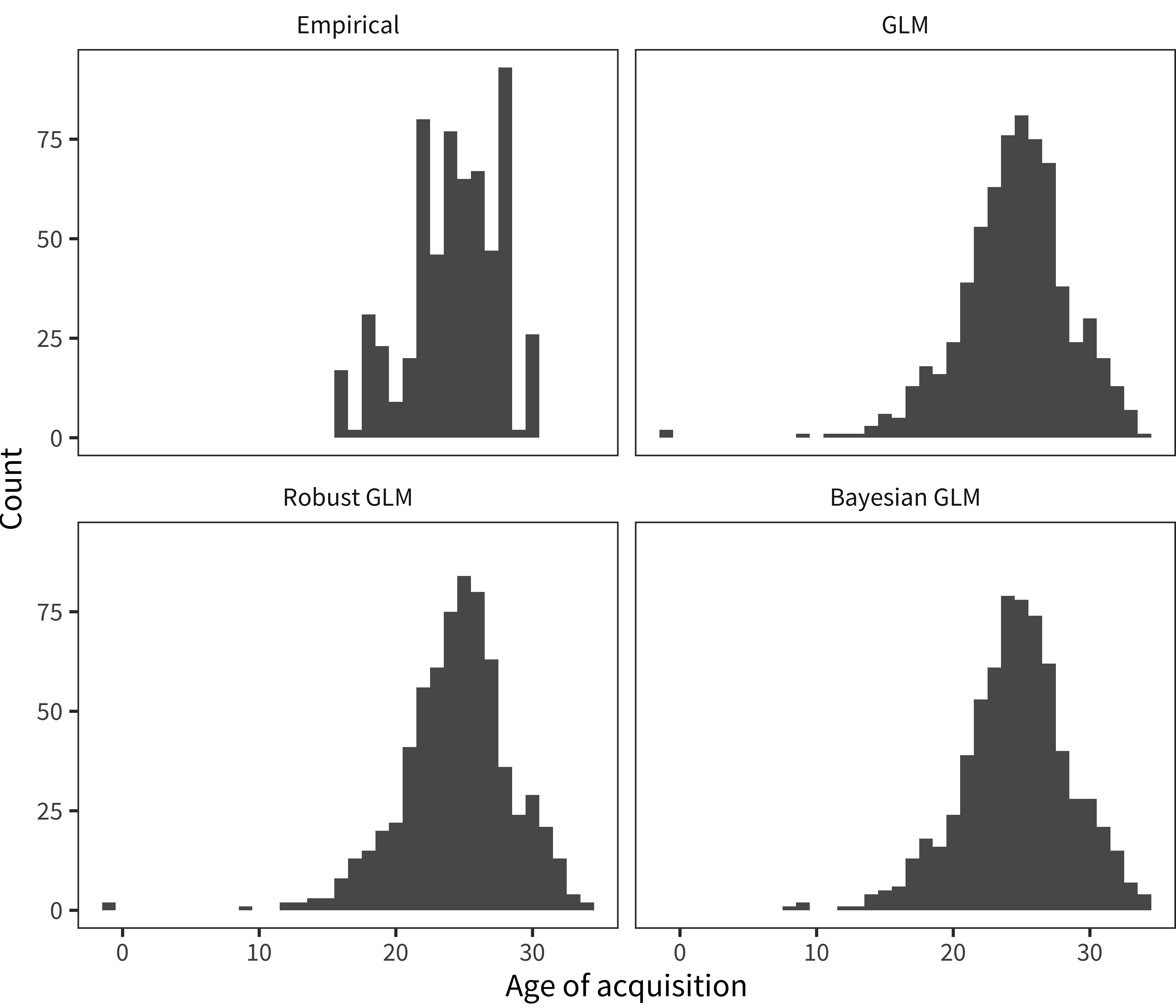
Figure D.1: Histogram of English (American) age of acquisition values as estimated via a variety of statistical methods (panels).
To further validate the Bayesian GLM approach, we tested the accuracy of the method in recovering AoAs for much smaller datasets. We did this by taking a subsample of only 100 children from the full English (American) WS dataset. We then fit standard and Bayesian GLMs to this sparse subsample. The resulting AoA estimates are plotted in Figure D.2. The Bayesian GLM shows the same minor bias to lower AoAs for hard words that the regular GLM does (a slightly below-diagonal slope), but the GLM shows noisier estimates for the earliest and (especially) the latest-learned words, suggesting that the regularization from the prior values in the Bayesian model is allowing it to deal with sparse data more effectively.
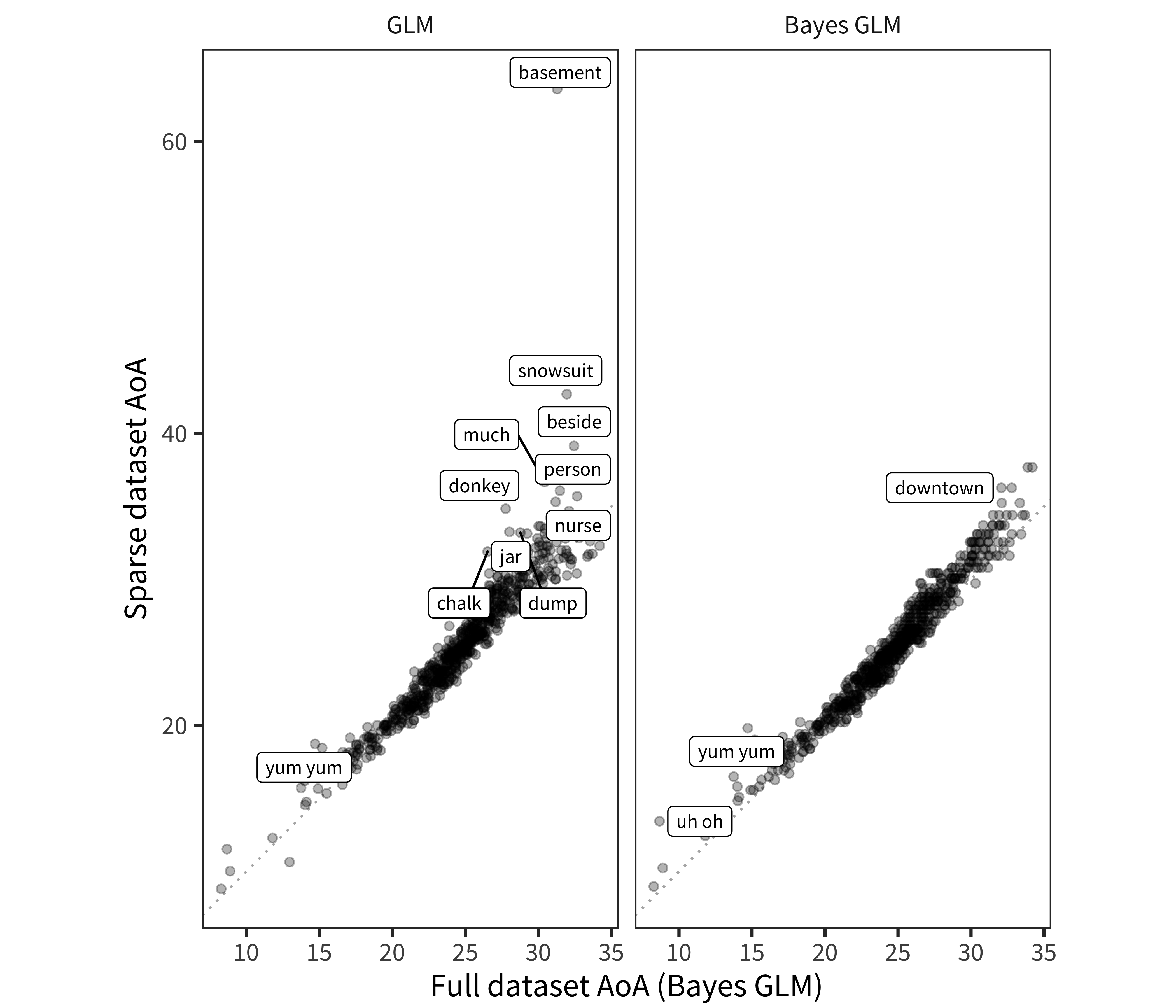
Figure D.2: Recovered AoAs from a sparse subsample (100 children), plotted by the Bayesian GLM AoAs from the full dataset. Left panel shows standard GLM, right panel shows Bayesian GLM. Differences of AoA > 4 months between methods are labeled.
In sum, our analyses here suggest that a Bayesian approach is useful for estimating AoA values.