Chapter 10 Predictive Models of the Acquisition of Individual Words
- Note:
- The contents of this chapter are lightly adapted from Braginsky et al. (2019).
In this chapter, we take up the challenge posed in Chapter 8, that is, to explain consistency and variability in the acquisition of individual words. Our approach is to define regression models that attempt to predict which words are learned earlier or later on the basis of a range of features drawn from different data sources. We fit these models to data across different languages and then interpret the resulting coefficients to draw conclusions about the potential contribution of different factors to children’s learning.
10.1 Introduction
As discussed in Chapter 1, one classic approach to word learning focuses on the specific mechanisms that children bring to bear on the learning problem. For example, across many laboratory experiments, a variety of mechanisms have been identified as plausible drivers of early word learning, including co-occurrence based and cross-situational word learning (Schwartz and Terrell 1983; C. Yu and Ballard 2007); social cue use (Baldwin 1993); and syntactic bootstrapping (Gleitman 1990; Mintz 2003). The individual contribution of each of these mechanisms has been difficult to assess, however.
Indeed, many theories of early word learning take multiplicity of cue types and mechanisms as a central feature (e.g., Hollich et al. 2000; Bloom 2000). As important as this work is, though, these studies are typically aimed at understanding how a small handful of words are learned in the laboratory under precisely-defined learning conditions. They do not directly address questions regarding the developmental composition and ordering of growth in the lexicon across many different children in their natural environments, nor whether these patterns are consistent across different languages.
An alternate approach to word learning – one that we have been following throughout this book – asks why some words are learned so early and some much later. This question about the order of the acquisition of first words can provide a different window into the nature of children’s language learning. In Chapter 8, we began approaching this question by examining the consistency of acquisition order for children’s earliest words. In the current chapter, we advance this goal using quantitative models to understand acquisition ordering.
Posed as a statistical problem, the challenge is to find what set of variables best predicts the age at which different words are acquired. This approach was pioneered by Huttenlocher et al. (1991) and developed further by Goodman, Dale, and Li (2008); it is now firmly established as an important method for understanding vocabulary learning at scale. This previous work has revealed that, in English, within a lexical category (e.g., nouns, verbs), words that are more frequent in speech to children are likely to be learned earlier (Goodman, Dale, and Li 2008). Further studies (also in English) have found evidence that age of acquisition is likely to be earlier for words that have more phonological neighbors (e.g., Storkel 2004; Stokes 2010; Jones and Brandt 2019; but see Swingley and Aslin 2007; Stager and Werker 1997); words that share more associations with other words in the learning environment (Hills et al. 2009); words that occur more often in isolation (Brent and Siskind 2001; Swingley and Humphrey 2018); words whose meanings are more concrete (Swingley and Humphrey 2018); words that are rated more iconic and/or more associated with babies (such as “choo-choo” or “doggy”, Perry, Perlman, and Lupyan 2015); and words that occur in more distinctive spacial, temporal, and linguistic contexts (Roy et al. 2015).
Each of these studies used a different dataset and focused on different predictors, however. In addition, nearly all analyzed data from English-learning children, providing no opportunity for cross-linguistic comparison of the relative importance of the many relevant factors under consideration. In this chapter, we extend these approaches and assess the degree to which the predictors of word learning are consistent across different languages and cultures, as well as whether there are similar patterns across different word types (e.g., nouns vs. verbs).
We conduct cross-linguistic comparisons of the age of acquisition of particular words. We integrate estimates of words’ acquisition trajectories from the Wordbank data with independently-derived characterizations of the word learning environment from other datasets. The use of secondary datasets for these analyses is warranted because no currently available resource provides data on both children’s language environments and their learning outcomes for more than a small handful of children. In particular, we derive our estimates of the language environment from transcripts of speech to children in the CHILDES database (MacWhinney 2000). This data-integration methodology was originated by Goodman, Dale, and Li (2008); it relies on large samples to average out the (substantial) differences between children and care environments. This is a conservative strategy because it requires substantial commonalities across families. While introducing additional sources of variability, it also allows for analyses that cannot be performed on smaller datasets or datasets that measure only child or environment but not both.
As our particular measures of environmental input, we estimated each word’s (a) frequency in parental speech to children, (b) mean length in words of the parental utterances containing that word (MLU-w), (c) frequency as a one-word utterance, and (d) frequency as the final word in an utterance. While these measures are crude, they are easy to compute and relatively comparable across the languages in our sample. To derive proxies for the meaning-based properties of each word, we accessed available psycholinguistic norms using adult ratings of each word’s (a) concreteness, (b) valence, (c) arousal, and (d) association with babies. Integrating these environmental and meaning-based measures, which are based respectively on estimates of children’s linguistic environment and words’ meaning, we predict each word’s acquisition trajectories. We assess the relative contributions of each predictor, as well as how those predictors change over development and interact with the lexical category of the word being predicted.
These analyses address two questions. First, we ask about the degree of consistency across languages in the relative importance of each predictor. Consistency in the patterning of predictors would suggest that similar information sources are important for learners, regardless of language. Such evidence would suggest that superficial linguistic dissimilarities (e.g., greater morphological complexity in Russian and Turkish, greater phonological complexity in Danish) do not dramatically alter the course of acquisition. Conversely, variability would show the degree to which learners face different challenges in learning different languages, posing a challenge for more universalist accounts. Further, systematicity in the variability between languages would reveal which languages are more similar than others in the structure of these different challenges.
Second, we ask which lexical categories are most influenced by specific linguistic environment factors, like frequency and utterance length, compared with meaning-based factors like concreteness and valence. Division of dominance theory suggests that nouns might be more sensitive to meaning factors, while predicates and closed-class words might be more sensitive to linguistic environment factors (Gentner and Boroditsky 2001). Following syntactic bootstrapping theories (Gleitman 1990), nouns are argued to be learned via frequent co-occurrence patterns in the input (operationalized by frequency) while verbs might be more sensitive to syntactic factors (operationalized here by utterance length; Snedeker, Geren, and Shafto 2007). Thus, examining the relative contribution of different predictors across lexical categories can help test the predictions of influential theories of acquisition.
10.2 Methods
10.2.1 Acquisition trajectories
Since analyses in this chapter rely on unilemma mappings (see Section 3.1.5), the set of languages represented is smaller than in other chapters. We use data from the items on WG forms for our comprehension measure, and data from the items in common between WG and WS forms for our production measure. Placeholder items, such as “child’s own name,” are excluded, as are longitudinal administrations. Table 10.1 gives an overview of our acquisition data.
| Language | Items | N | Ages | N | Ages | Types | Tokens |
|---|---|---|---|---|---|---|---|
| Croatian | 388 | 627 | 8-30 | 250 | 8-16 | 12,064 | 218,775 |
| Danish | 381 | 6,112 | 8-36 | 2,398 | 8-20 | 4,956 | 195,658 |
| English | 393 | 7,312 | 8-30 | 1,792 | 8-18 | 45,597 | 7,679,042 |
| French | 396 | 1,364 | 8-30 | 537 | 8-16 | 28,819 | 2,551,113 |
| Italian | 392 | 1,400 | 7-36 | 648 | 7-24 | 7,544 | 188,879 |
| Norwegian | 380 | 7,466 | 8-36 | 2,374 | 8-20 | 10,670 | 231,763 |
| Russian | 410 | 1,805 | 8-36 | 768 | 8-18 | 5,191 | 32,398 |
| Spanish | 399 | 1,891 | 8-30 | 788 | 8-18 | 33,529 | 1,609,614 |
| Swedish | 371 | 1,367 | 8-28 | 467 | 8-16 | 8,815 | 359,155 |
| Turkish | 395 | 3,537 | 8-36 | 1,115 | 8-16 | 6,503 | 44,347 |
See Figure 10.1 for example smoothed empirical item curves of the type being predicted in our subsequent analyses.
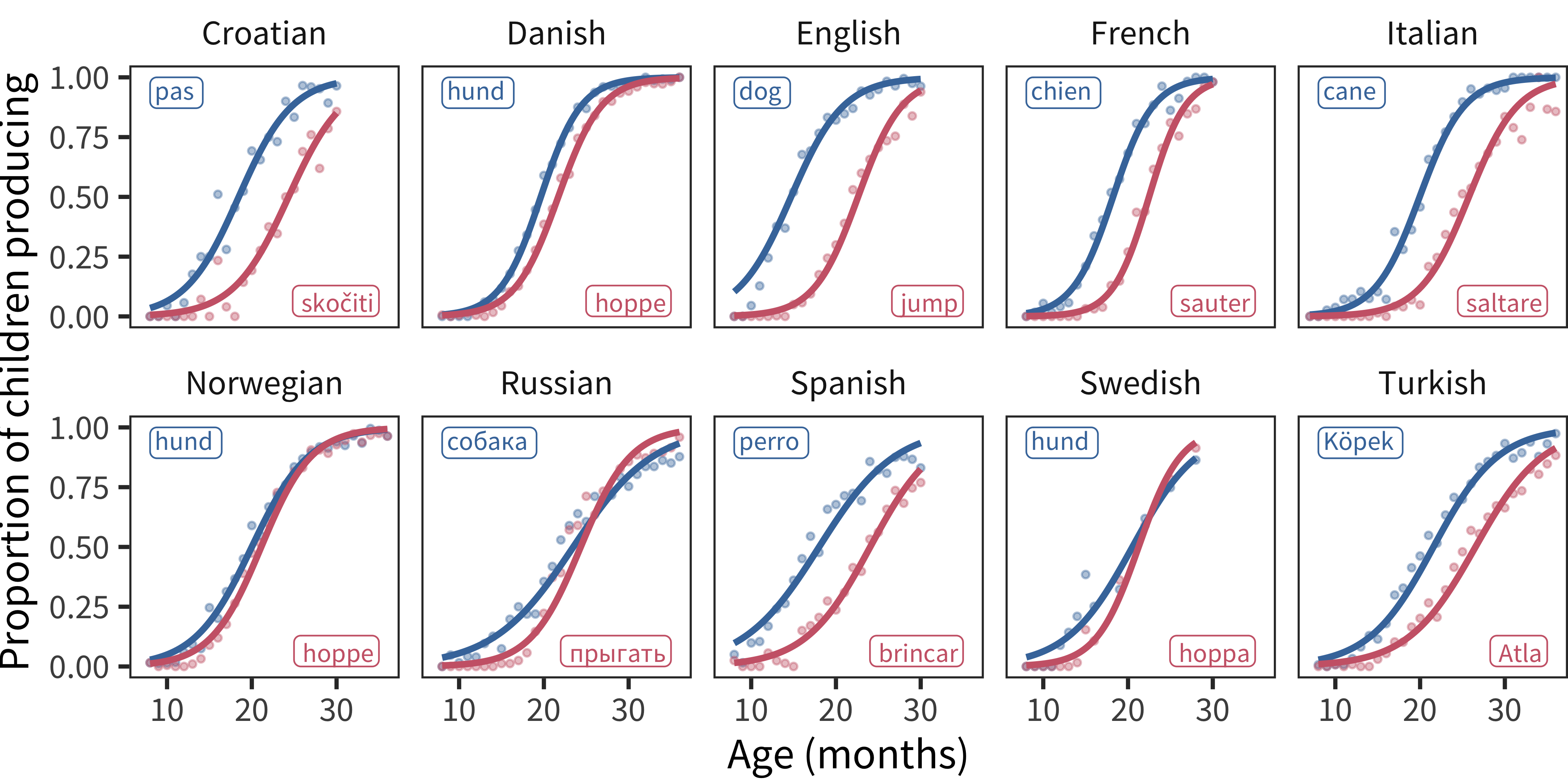
Figure 10.1: Example production trajectories for the words “dog” and “jump” across languages. Points show the proportion of children producing each word for each one-month age group. Lines show the best-fitting logistic curve. Labels show the forms of the words in each language.
10.2.2 Word properties
For each word that appears on the forms in each of our 10 languages, we used corpora of child-directed speech in that language from CHILDES to obtain an estimate of its frequency, the mean length of utterances in which it appears, its frequency as the sole constituent of utterance, and its frequency in utterance final position (with frequency residualized out of solo and final frequencies). Additionally, we computed each word’s length in phonemes.
To capture meaning-based factors in acquisition, we included ratings of each word’s concreteness, valence, arousal, and relatedness to babies. All of these ratings were compiled based on previous studies using adult raters. In addition, since existing datasets for all of these ratings are primarily available for English, we used the unilemma mappings (see Section 3.1.5) to use the ratings for English words across languages. Example words for these predictors in English are shown in Table 10.2.
| Predictor | Lowest | Highest |
|---|---|---|
| Arousal | today, asleep, shh | naughty, money, scared |
| Babiness | jeans, penny, donkey | baby, bib, bottle |
| Concreteness | that, now, how | apple, baby, ball |
| Final frequency | put, when, give | book, it, there |
| Frequency | babysitter, rocking chair, grrr | you, it, that |
| MLU | ouch, thank you, peekaboo | daddy, when, day |
| Number phonemes | i, eye, ear | refrigerator, cockadoodledoo, babysitter |
| Solo frequency | feed, bathroom, tooth | no, yes, thank you |
| Valence | ouch, hurt, sick | happy, hug, love |
Previous studies have shown robust consistency in the types of words that children learn very early (Tardif et al. 2008). These words seem to describe concepts that are important or exciting in the lives of infants in a way that standard psycholinguistic features like concreteness do not. Capturing this intuition quantitatively is difficult, but Perry, Perlman, and Lupyan (2015) provides a proxy measure as a first step. This measure is simply the degree to which a particular word was “associated with babies.” Intuitively, we expect this measure to capture the degree to which words like ball or bottle feature heavily in the environment (and presumably, mental life) of many babies.
Each numeric predictor was centered and scaled so that all predictors would have comparable units.
Frequency. For each language, we estimated word frequency from unigram counts based on all corpora in CHILDES for that language (all corpora from a given language were included, regardless of dialect). Frequencies varied widely both within and across lexical categories. Each word’s count includes the counts of words that share the same stem (so that dogs counts as dog) or are synonymous (so that father counts as daddy). For polysemous word pairs (e.g., orange as in color or fruit), occurrences of the word in the corpus were split uniformly between the senses on the CDI (there were only between 1 and 10 such word pairs in the various languages; in the absence of cross-linguistic corpus resources for polysemy sense disambiguation, this is a necessary simplification). Counts were normalized to the length of each corpus, Laplace smoothed (i.e., count of 0 were replaced with counts of 1), and then log transformed.
Solo and Final Frequencies. Using the same dataset as for frequency, we estimated the frequency with which each of word occurs as the sole word in an utterance, and the frequency with which it appears as the final word of an utterance (not counting single-word utterances). As with frequency, solo and final counts were normalized to the length of each corpus, Laplace smoothed, and log transformed. Since both of these estimates are by necessity highly correlated with frequency, we then residualized unigram frequency out of both of them, so that values reflect an estimate of the effects of solo frequency and final frequency over and above frequency itself.
MLU-w. MLU-w is only a rough proxy for syntactic complexity, but is relatively straightforward to compute across languages (in contrast to other metrics). For each language, we estimated each word’s MLU-w by calculating the mean length in words of the utterances in which that word appeared, for all corpora in CHILDES for that language. For words that occurred fewer than 10 times, MLU-w estimates were treated as missing.
Number of phonemes. In the absence of consistent resources for cross-linguistic pronunciation, we computed the number of phonemes in each word in each language based on phonemic transcriptions of each word obtained using the eSpeak tool (Duddington 2012). We then spot-checked these transcriptions for accuracy.
Concreteness. We used previously collected norms for concreteness (Brysbaert, Warriner, and Kuperman 2014), which were gathered by asking adult participants to rate how concrete the meaning of each word is on a 5-point scale from abstract to concrete.
Valence and Arousal. We also used previously collected norms for valence and arousal (Warriner, Kuperman, and Brysbaert 2013), for which adult participants were asked to rate words on a 1-9 happy-unhappy scale (valence) and 1-9 excited-calm scale (arousal).
Babiness. Lastly, we used previously collected norms of “babiness”, a measure of association with infancy (Perry, Perlman, and Lupyan 2015) for which adult participants were asked to judge a word’s association with babies on a 1-10 scale.
Lexical category. Category was determined on the basis of the conceptual categories presented on the CDI form (e.g., “Animals”, “Action Words”), such that the Nouns category contains common nouns, Predicates contains verbs and adjectives, and Function Words contains closed-class words (following Bates et al. 1994), and the remaining items are binned as Other.
Imputation. The resulting sets of predictor values for each language had varying numbers of missing values, depending on resource availability (number phonemes 0%, concreteness 0%-1%, arousal and valence 8%-13%, [solo/final] frequency 2%-14%, babiness 10%-33%, MLU-w 2%-53%). We used iterative regression imputation to fill in these missing values (separately within each language) by first replacing missing values with samples drawn randomly with replacement from the observed values, and then iteratively imputing values for a predictor based on a linear regression fitting that predictor from all others.
Collinearity. A potential concern for comparing coefficient estimates is predictor collinearity. Fortunately, in every language, the only relatively large correlations are between MLU-w and solo frequency (mean over languages r = –0.44), as expected given the similarity of these factors, along with modest correlations between frequency and concreteness (mean over languages r = –0.36) and between frequency and number of phonemes (mean over languages r = –0.33), a reflection of Zipf’s Law (Zipf 1935). More importantly, the variance inflation factor for each of the predictors in each language is no greater than 2.3, indicating that multicollinearity among the predictors is low.
10.2.3 Analysis
We used mixed-effects logistic regression models (fit with the MixedModels package in Julia; Bates et al. 2018) to predict whether each child understands/produces each word from the child’s age, properties of the word, interactions between each property and age, and interactions between each property and lexical category (which was contrast coded). Each model was fit to all data from a particular language and included a random intercept for each word and a random slope of age for each word. Computational and technical limitations prevented us from including random effects for child or including data from all languages in one joint model.
The magnitude of the standardized coefficient on each property gives an estimate of its independent contribution to words being understood/produced by more children. Interactions between properties and age give estimates of how this effect is modulated for earlier-learned and later-learned words. For example, a positive effect of babiness means that words associated with babies are known by more children; a negative interaction with age means that high babiness leads to higher rates of production and comprehension for younger children compared with older children. Similarly, interactions between properties and lexical category give estimates of how the effect differs among nouns, predicates, and function words.
10.3 Results
English predictor effects. To illustrate the structure of our analysis, we first describe the results for English data, shown in Figure 10.2 as the main effect and age interaction coefficient estimates and 95% confidence intervals, for comprehension and production. For main effects, words are more likely to be known by more children if they are higher in frequency or concreteness, as well as in babiness for comprehension and in sentence-final frequency or sole-constituent frequency for production. In contrast, words that appear in shorter sentences (MLU-w) are more likely to be reported as understood or produced. For age interactions, while most predictors have consistent effects over age, words that are higher in frequency or concreteness are more likely to be known more by older children, while words that are higher in valence have a greater effect on acquisition in younger children, with an additional negative interaction with babiness in comprehension and positive interaction with MLU-w in production.
Cross-linguistic predictor effects. Figure 10.3 shows the coefficient estimate for each predictor in each language and measure. We find that frequency is the strongest predictor of acquisition (mean across languages and measures \(\beta\) = 0.23). Other relatively strong overall predictors include concreteness (\(\beta\) = 0.18), solo frequency (\(\beta\) = 0.17), MLU-w (\(\beta\) = –0.14), and final frequency (\(\beta\) = 0.13). Number of phonemes is comparatively large for production (\(\beta\) = –0.31) but not comprehension (\(\beta\) = –0.07); conversely, babiness is comparatively large for comprehension (\(\beta\) = 0.19) but not production (\(\beta\) = 0.08). Finally, valence (\(\beta\) = 0.06) and arousal (\(\beta\) = 0.003) have much smaller effects.
Given the emphasis on frequency effects in the literature (Ambridge et al. 2015), one might have expected frequency to dominate, but several other predictors are also quite strong. In addition, some factors previously argued to be important for word learning, namely valence and arousal (Moors et al. 2013), appear to have limited relevance when compared to other factors. These results provide a strong argument for our approach of including multiple predictors and languages in our analysis.
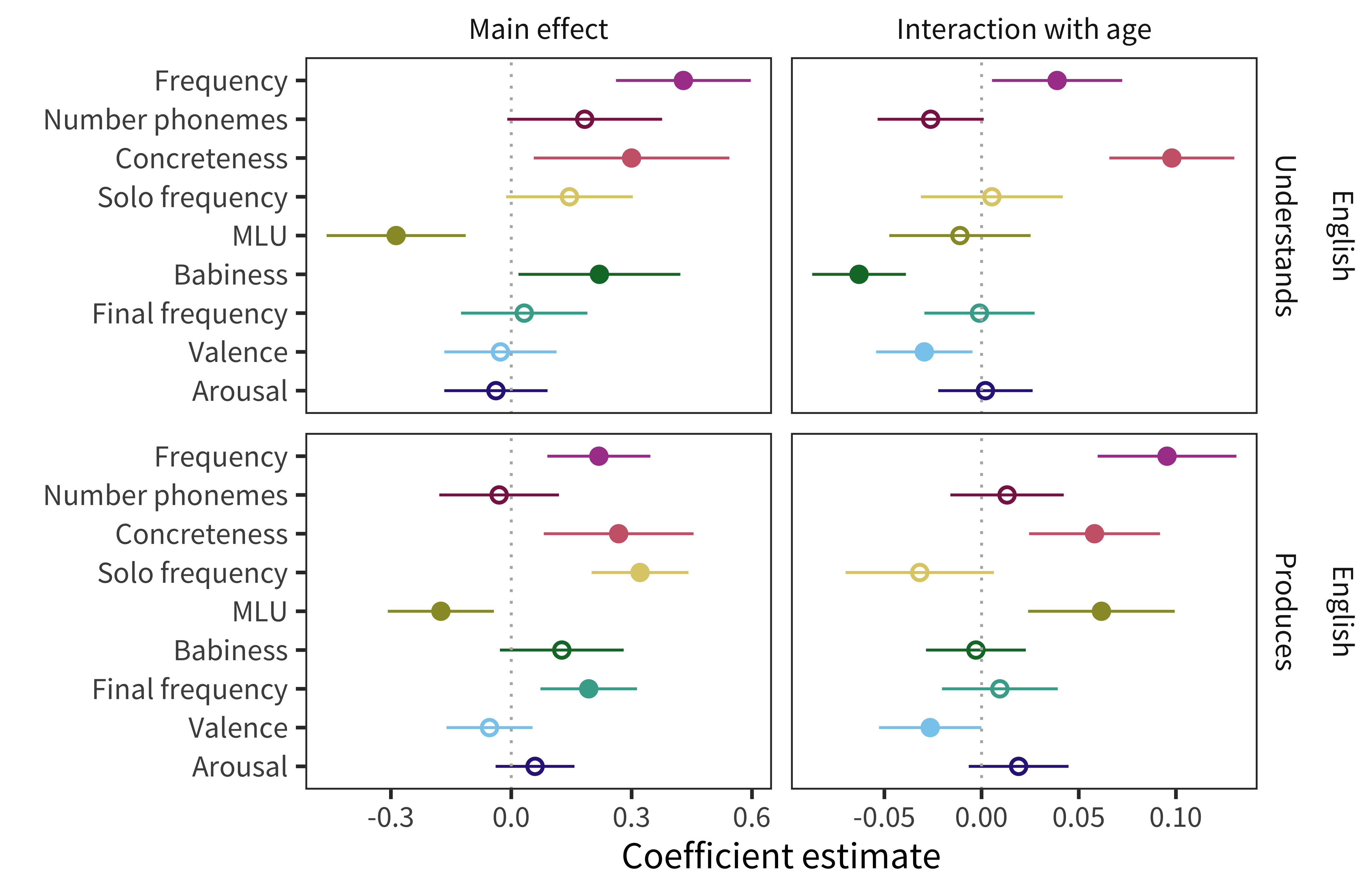
Figure 10.2: Estimates of coefficients in predicting words’ developmental trajectories for English comprehension and production data. Error bars indicate 95% confidence intervals; filled in points indicate coefficients for which p < 0.05.
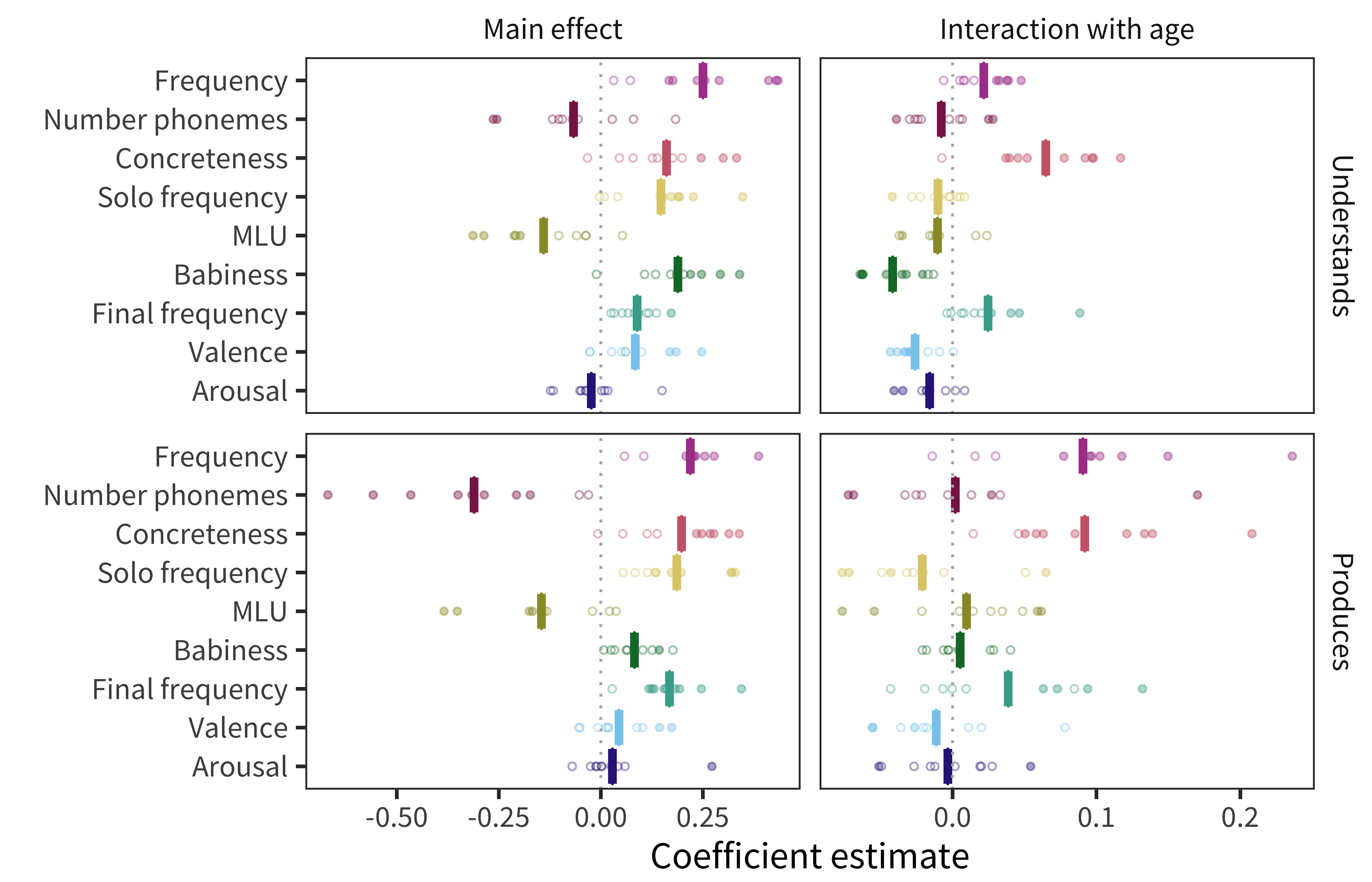
Figure 10.3: Estimates of coefficients in predicting words’ developmental trajectories for all languages and measures. Each point represents a predictor’s coefficient in one language, with the bar showing the mean across languages. Filled in points indicate coefficients for which p < 0.05.
Consistency. Apart from valence and arousal, all other predictors have the same the direction of effect in all or almost all languages and measures (at least 17 of the 20). Thus, across languages, words are likely to be understood and produced by more children if they are more frequent, shorter, more concrete, more frequently the only word in an utterance, more associated with babies, more frequently the final word in an utterance, and appear in shorter utterances.
Additionally, there is considerable consistency in the magnitudes of predictors across languages. A priori, it could have been the case that different languages have wildly different effects of various factors (due to linguistic or cultural differences), but this pattern is not what we observe. Instead, there is more consistency in the correlations between coefficients across languages than would be expected by chance. As shown in Figure 10.4, each language’s mean pairwise correlation with other languages’ coefficients (i.e., the correlation of coefficients for English with coefficients for Russian, for Spanish, and so on) is outside of bootstrapped estimates in a randomized baseline created by shuffling predictor coefficients within language. The pairwise correlations are more consistent for production (mean r = 0.72) than for comprehension (mean r = 0.56), in which French and Russian effects are more idiosyncratic.
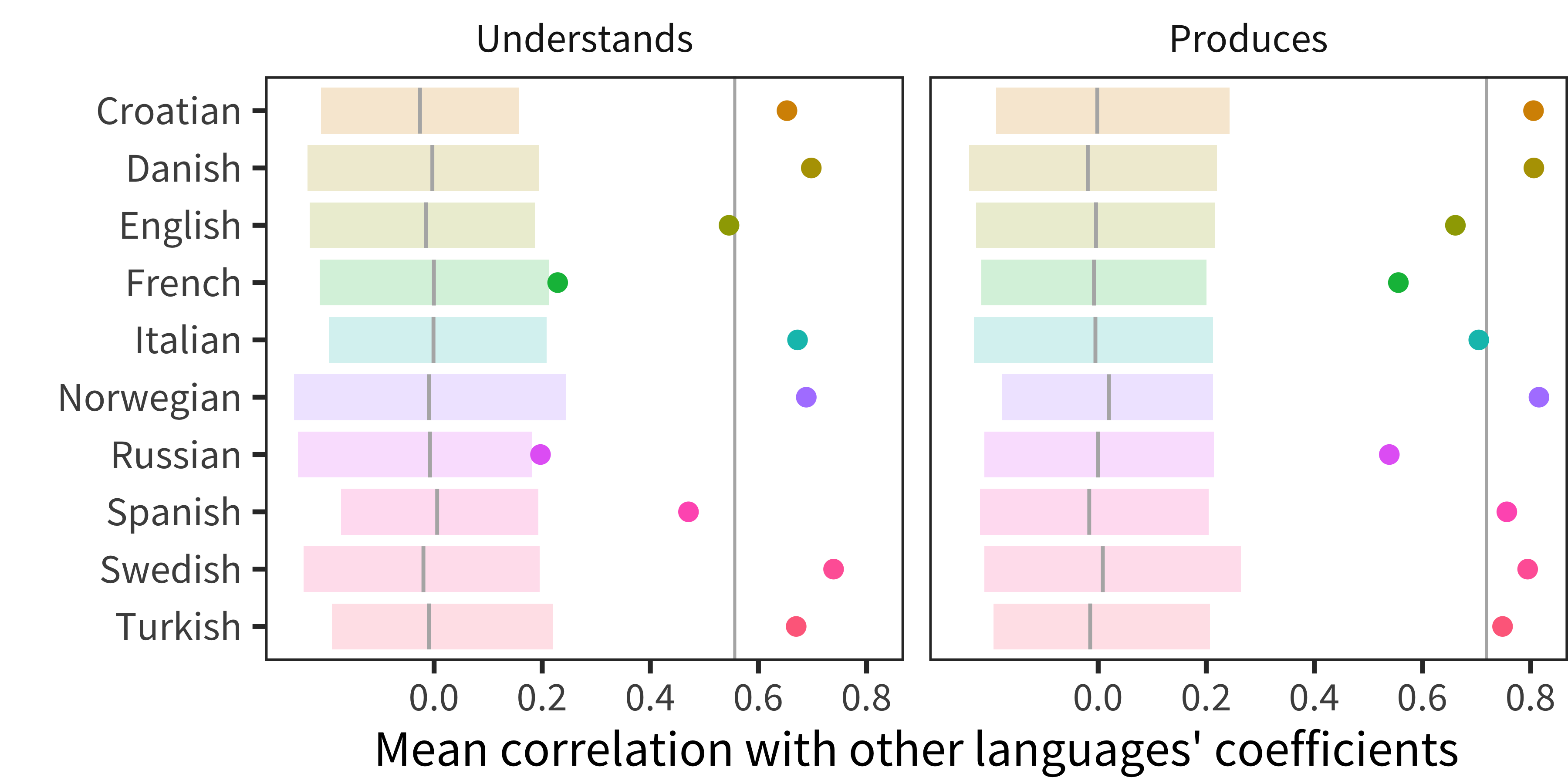
Figure 10.4: Correlations of coefficient estimates between languages. Each point represents the mean of one language’s coefficients’ correlation with each other language’s coefficients, with the vertical line indicating the overall mean across languages. The shaded region and line show a bootstrapped 95% confidence interval of a randomized baseline where predictor coefficients are shuffled within language.
Variability. While some particular coefficients differ substantially from the trend across languages (e.g., the effect of frequency for comprehension in Spanish is near 0), these individual datapoints are difficult to interpret. Many unmeasurable factors could potentially account for these differences: Spanish frequency estimates could be less accurate due to corpus sparsity or idiosyncrasy, the samples of children in the Spanish CDI and CHILDES data could differ more demographically, or Spanish-learning children could in fact rely less on frequency. Rather than attempting to interpret individual coefficients, we instead ask how the patterns of difference among languages reflect systematic substructure in the variability of the effects.
To examine the substructure of predictor variability, we followed Chapter 8 in using hierarchical clustering analysis to find the similarity structure among the pairwise correlations between languages’ predictors. The resulting dendrograms are shown in Figure 10.5, which broadly reflect language typology, especially for production data. This result suggests that some language-to-language similarity is captured by the profile of coefficient magnitudes our analysis returns.
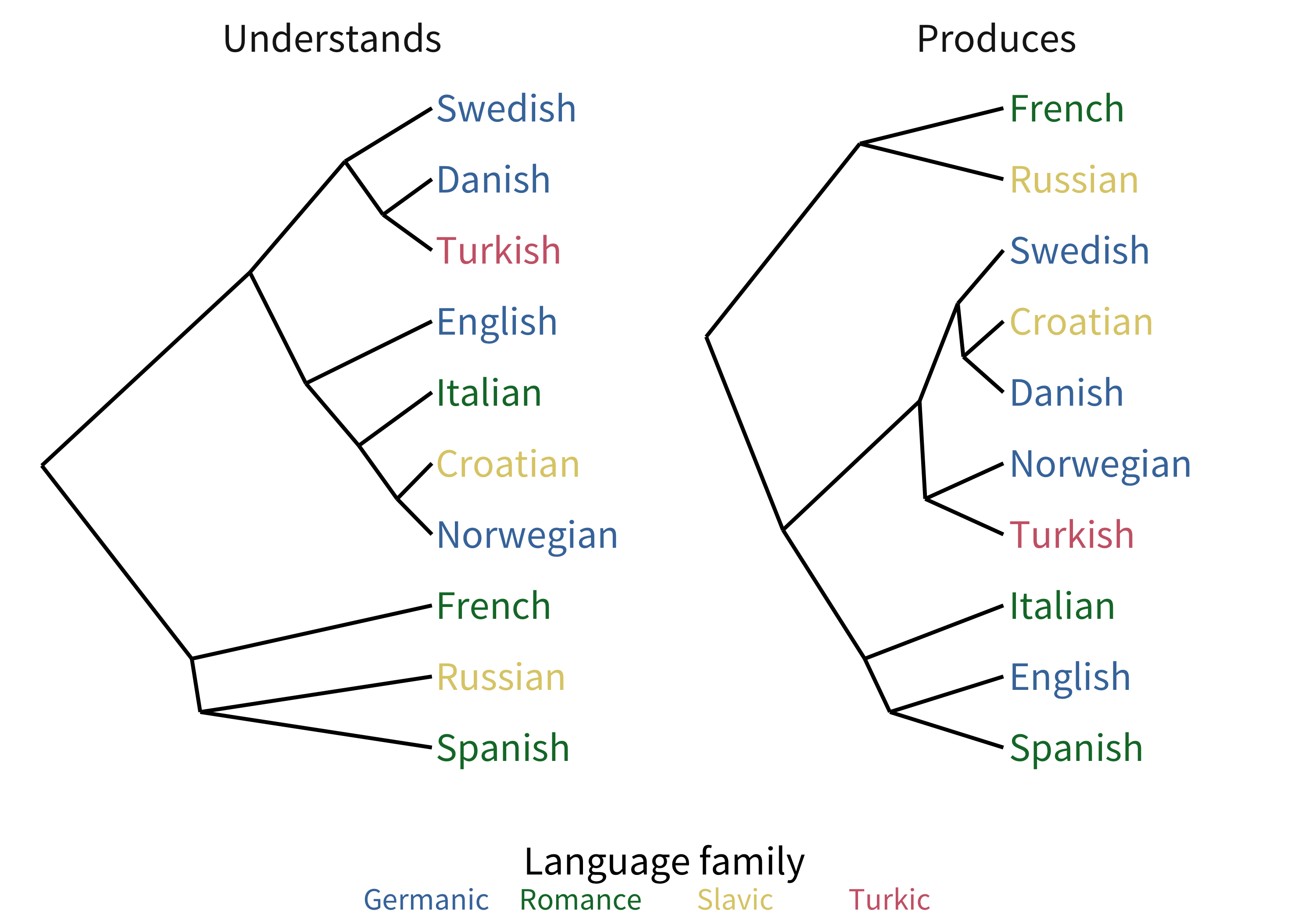
Figure 10.5: Dendrograms of the similarity structure among languages’ coefficients.
Comprehension vs. production. As mentioned above, word length is the one predictor of acquisition that varies substantially between measures: it is far more predictive for production than for comprehension. Although not all children will produce precisely the citation form of CDI words, words that have longer citation forms will also on average tend to have more difficult realizations in child language (e.g., although some children will say “raf” for “giraffe,” others will attempt the full citation form). Given this, as measured here, length seems to reflect effects of production constraints (i.e., how difficult a word is to say) rather than comprehension constraints (i.e., how difficult it is to store or access). This result may explain why the hierarchical clustering analysis above appears more similar to linguistic typology in production than comprehension, that is, the role of production difficulty may be more similar for more typologically-related languages. Another possibility is that since the measures are confounded with age (comprehension is only measured for younger children), word length may play a larger role later in acquisition. Similarly, the stronger effect of babiness in comprehension over production could be due to its larger prominence earlier in development.
Developmental change. For both comprehension and production, positive age interactions can be seen in at least 9 out of 10 languages for concreteness and frequency. Conversely, there are negative age interactions for babiness and valence for comprehension in at least 9 out of 10 languages. This suggests that concreteness and frequency facilitate learning more so later in development, while babiness and valence facilitate learning earlier in development. This result is consistent with the speculation above that the babiness predictor captures meanings that have special salience to very young infants.
Lexical categories. Previous work suggests that predictors’ relationship with age of acquisition differs among lexical categories (Goodman, Dale, and Li 2008). We investigate these differences by including lexical category interaction terms in our model. Figure 10.6 shows the resulting effects for each lexical category, combining the main effect of a given predictor with the main effect of the lexical category and the interaction between that predictor and that lexical category.
Across languages, the strongest predictors of acquisition for both nouns and predicates are concreteness (nouns \(\beta\) = 0.44; predicates \(\beta\) = 0.28) and frequency (nouns \(\beta\) = 0.36; predicates \(\beta\) = 0.41). Thus content words are most likely to be known by more children if they are more frequent or more concrete. Conversely, function words are most influenced by number of phonemes (\(\beta\) = –0.74), babiness (\(\beta\) = –0.61), and MLU-w (\(\beta\) = –0.61), meaning that function words are most likely to be known by more children if they are shorter, less associated with babies, or appear in shorter sentences. These patterns are supportive of the hypothesis that different word classes are learned in different ways, or at least that the bottleneck on learning tends to be different, with different information sources having varying degrees of relevance across categories.
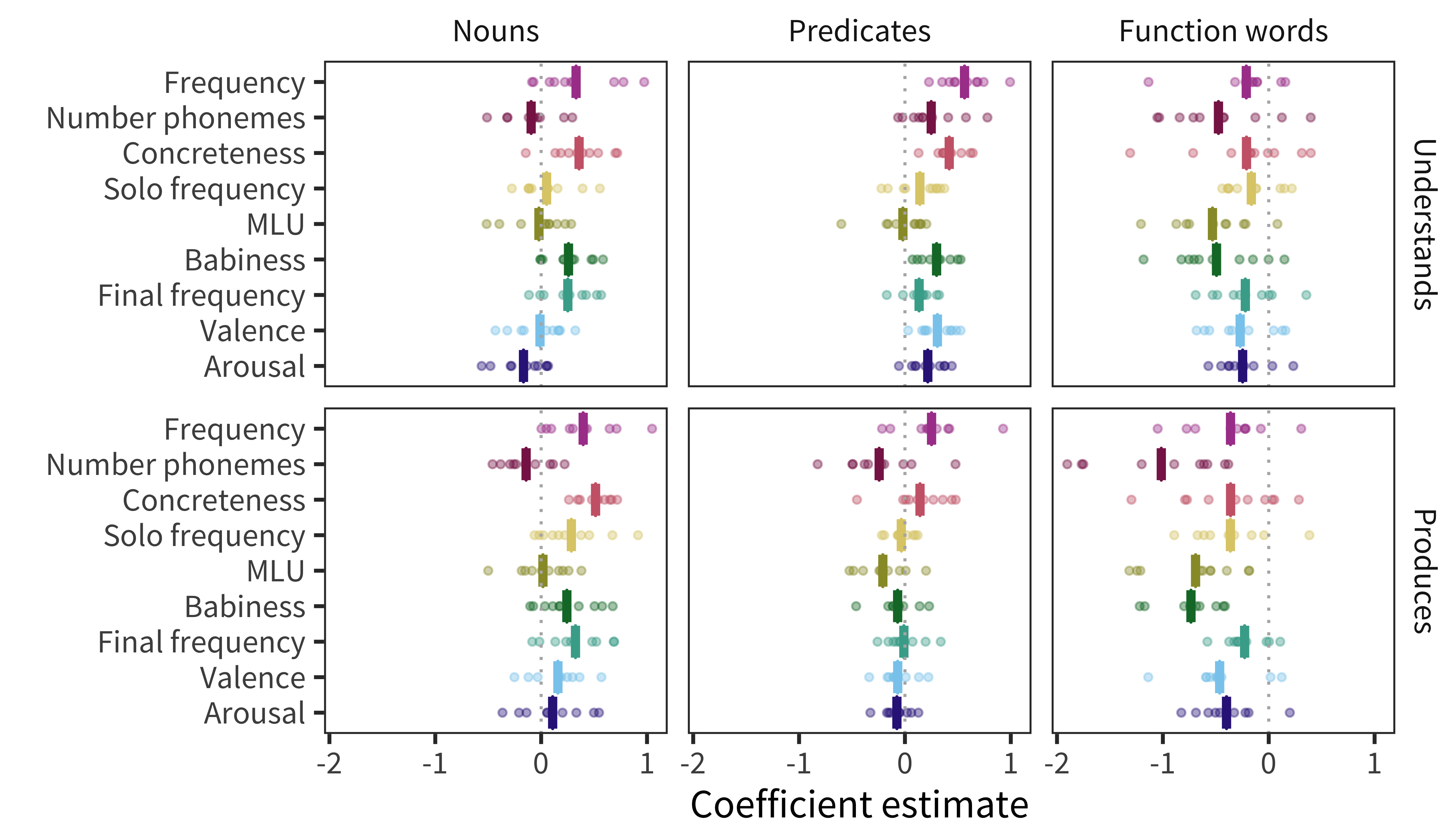
Figure 10.6: Estimates of effect in predicting words’ developmental trajectories for each language, measure, and lexical category (main effect of predictor + main effect of lexical category + interaction between predictor and lexical category). Each point represents a predictor’s effect in one language, with the bar showing the mean across languages.
Additionally, the mean pairwise correlation of coefficients between languages is much larger for nouns (r = 0.68) and predicates (r = 0.54) than for function words (r = 0.29). The higher between-language variability for function words suggests the learning processes differ substantially more across languages for function words than they do for content words.
10.4 Discussion
What makes words easier or harder for young children to learn? Previous experimental work has largely addressed this question using small-scale lab studies. While such experiments can identify sources of variation, they typically do not allow for different sources to be compared directly. In contrast, observational studies allow the effects of individual factors to be measured across ages and lexical categories (e.g., Goodman, Dale, and Li 2008; Hills et al. 2009; Swingley and Humphrey 2018), but are limited in the size and scope of the datasets and languages that can be directly compared. We derived several new findings from our analyses, in part due to the larger set of languages and predictors we were able to include.
First, we found consistency in the patterning of predictors across languages at a level substantially greater than the predictions of a chance model. This consistency supports the idea that differences in culture or language structure do not lead to fundamentally different acquisition strategies, at least at the level of detail we were able to examine. Instead, they are likely produced by processes that are similar across populations and languages. We return to a discussion of these “process universals” in Chapter 17.
Second, predictors varied substantially in their weights across lexical categories. Frequent, concrete nouns were learned earlier, consistent with theories that emphasize the importance of early referential speech (e.g., Baldwin 1995). For predicates, concreteness was somewhat less important and frequency some more important. And for function words, length and MLU-w was more predictive, perhaps because it is easiest to decode the meanings of function words that are used in short sentences (or because such words have meanings that are easiest to decode). Overall, these findings are consistent with some predictions of both division of dominance theory, which highlights the role of conceptual structure in noun acquisition (Gentner and Boroditsky 2001), and syntactic bootstrapping theory, which emphasizes linguistic structure over conceptual complexity in the acquisition of lexical categories other than nouns (Snedeker, Geren, and Shafto 2007). More generally, our methods here provide a way forward for testing the predictions of these theories across languages and at the level of the entire lexicon rather than individual words.
In addition to these new insights, several findings emerged that confirm and expand previous reports. Environmental frequency was an important predictor of learning, with more frequently-heard words learned earlier (Goodman, Dale, and Li 2008; Swingley and Humphrey 2018). Predictors also changed in relative importance across development. For example, certain words whose meanings were more strongly associated with babies appeared to be learned early for children across the languages in our sample – perhaps explaining our findings in Chapter 8 (see also Tardif et al. 2008). Finally, word length showed a dissociation between comprehension and production, suggesting that challenges in production do not carry over to comprehension (at least in parent-report data).