Chapter 15 Individual Variation in Vocabulary
Of all the individual differences described to date in the literature on early child language, variations in rate present the least interesting challenge to traditional ‘universalist’ models of development. If it can be shown that all children go through the same basic sequence, activating a common set of structures and processes, then small variations in the onset time for specific language milestones might represent little more than a minor perturbation to a maturational theory (like variations in the onset of puberty). Putative variations in style of development are more problematic, because they raise questions about the order in which structures are acquired, and the mechanisms used to acquire those structures. (Bates et al. 1994, 86)
Preceding chapters have dealt with the degree of variability in vocabulary size between individuals in Chapter 5 and the stability of individuals’ percentile rank in Chapter 4. Then Chapters 6 and 9 explored demographic factors as (partial) explanations of this variability. Throughout, our treatment of variability has focused on issues of learning rate in the sense discussed by Bates et al. in the quote above. With the exception of Chapter 9, which examined the rate of learning individual words, we have not dealt yet with issues of style. This chapter rectifies that omission, investigating three major topics: (1) whether there is stable individual variation in the category composition of vocabulary, (2) whether there are “spurts” in vocabulary growth, and (3) whether there is stable variation in the relationship between production and comprehension. To summarize, our answers are “yes,” “no,” and “difficult to determine,” respectively.
15.1 Introduction
What does it mean for two children to show differences in language learning style? Intuitively, children who vary in style of learning should differ in some aspect(s) of the learning process. Unfortunately, from the data that we use here, we cannot observe process – we can only observe the outcome of learning: knowledge. Thus, children must exhibit some differences in the way their vocabulary grows. This difference could be distributional and inferred indirectly from cross-sectional data or it could be shown directly through longitudinal data (though this strategy limits the number of datasets we can use from Wordbank).
One prominent candidate for a stylistic difference in language acquisition is the distinction between “referential” and “expressive” children. In an early report on individual differences in vocabulary acquisition, Nelson (1973) noticed that there was substantial variation in how many nouns children had in their vocabularies. Children who had more than half of their vocabulary devoted to nouns were named “referential” children. They tended to have speech that was less syntactically complex than other children and showed faster vocabulary growth. In contrast, “expressive” children had speech that was more syntactically complex and had fewer nouns. Dore (1974) proposed a related version of this distinction, focusing on speech acts from two children in the middle of the second year and labeling them as “code oriented” (focused on labeling, similar to “referential”) vs. “message oriented” (instrumental, social requests, similar to “expressive”).
Since this seminal work, the referential/expressive distinction has become enshrined in the literature as a canonical aspect of variation in children’s style. Yet further debate about the consequences of this stylistic distinction continued in the literature. For example, Bates, Bretherton, and Snyder (1988) observed a correlation between the proportion of nouns in the children’s vocabulary and their vocabulary size and suggested the possibility that referential style might simply reflect a more effective strategy for learning. Reacting to this claim, Pine and Lieven (1990) argued that the direction of causality might be reversed, however: perhaps having a bigger vocabulary (at least at a certain point) would lead to a greater representation for nouns.28
While exploring the referential/expressive phenomenon more rigorously, Bates et al. (1994) presented analyses largely supporting the Pine and Lieven view: much systematic variation in the “referentiality” (proportion nouns) in children’s vocabularies was due to the size of their vocabulary. As children’s vocabularies grow, they tend to increase in their over-representation of nouns (as shown also in Chapter 11). Thus, two children of the same age who have different proportions of nouns may also have different overall vocabulary sizes. After controlling for overall vocabulary size, Bates et al. (1994) found only limited evidence for stylistic variation. In the first subsection of this chapter, we pick up these analyses and apply them broadly to our dataset.
A second area of stylistic variation that has been much discussed is whether some children go through a vocabulary “spurt,” defined as a change in the rate of vocabulary growth. The idea of a “spurt” or “explosion” occurs in a wide variety of discussions of early vocabulary (e.g., Nelson 1973; Kamhi 1986; Bates, Bretherton, and Snyder 1988; see e.g., Dapretto and Bjork 2000 for review). Clearly, from the average growth rates observed in Chapter 5, children’s vocabulary growth accelerates dramatically during the period following their first birthday and the emergence of first word production. Investigations of this acceleration have focused on two distinct issues: its explanation and its variation across children.
Although there has been a tremendous amount of discussion in the literature, we will not investigate the possible explanations of accelerations in vocabulary growth, i.e., the vocabulary spurt. Our data do not allow us to investigate issues of mechanistic process directly or of the cognitive or social changes which are co-contemporaneous with the vocabulary spurt. In addition, a short, but convincing, analysis by McMurray (2007) suggests that such acceleration is over-determined in the sense that it will likely emerge from almost any plausible acquisition mechanism(s). Assuming that words vary in difficulty as a normal distribution, vocabulary growth will naturally accelerate with increases in a child’s ability. Similar arguments have been made by Plunkett et al. (1992); see also Chapters 3 and 4 in Elman et al. (1996). Thus, making reverse inferences from the presence of acceleration to a particular mechanism is unwarranted.
The second issue – variation in acceleration across children – is related to our aims in this study, however. Does every child’s vocabulary acceleration follow the same general pattern, or is there substantial variation in the type of growth that is followed, for example, in the point at which acceleration begins, or the specific shape of the growth curve? Ganger and Brent (2004) report a systematic study of a sub-part of this issue: whether there is a discontinuity in growth rate for individual children. Defining a spurt specifically as a change in the rate of acceleration, they conducted a quantitative analysis of whether such a change occurs for all children using original data and data from several classic studies (Goldfield and Reznick 1990; Dromi 1987). Their results indicated that a change in rate of acceleration best captured the growth trajectories for only a small sub-set (only about 1 in 5) of the children analyzed. Our second set of analyses follows up on this general issue.
In the third section of this chapter, we address another stylistic issue, the dissociation between comprehension and production. It has been long acknowledged that children tend to understand more than they can say (e.g., Clark and Hecht 1983). But, to what extent does this generalization vary across children? That is, are there some children who understand many words who are also fluent producers vs. others who have a large vocabulary in comprehension but have more limited production? At the clinical extreme, significant variation in this respect must be present, because there are some children with various apraxias of speech that have strong comprehension but serious production difficulties. At the other extreme, delays in early comprehension have clinical relevance, and are often thought to be a more reliable indicator of language delays compared to production alone (e.g., Rescorla 2009; Thal, Tobias, and Morrison 1991). While both of these extremes are interesting and important, the question for us is whether, in a typically-developing population, we can detect, and possibly identify correlates of, systematic variation on this dimension over the full range of language abilities.
15.2 Variation in vocabulary composition
In this subsection we examine the question of variation across children in the degree to which their vocabularies reflect a “referential” vs. “expressive” style. Following Bates et al. (1994), we operationalize the notion of “referential” children as those with a relatively higher than average proportion of nouns compared to other children (the definition of “noun” is the same here as in Chapter 11. While there might be other more nuanced measures that we could construct, this one has the advantage of being directly related to the analysis framework utilized in Chapter 11; thus, we use that same framework to investigate vocabulary composition in individuals here.
15.2.1 Measuring vocabulary composition in individuals
The proportion of children’s vocabulary that is made up of nouns is shown in Figure 15.1. There is a general trend for an over-representation of nouns, as shown by the blue line (representing the smoothed mean proportion nouns) being above the red dashed line (total proportion nouns on the form). The size of this over-representation across languages is the topic of Chapter 11. Here, we examine its variability across children.
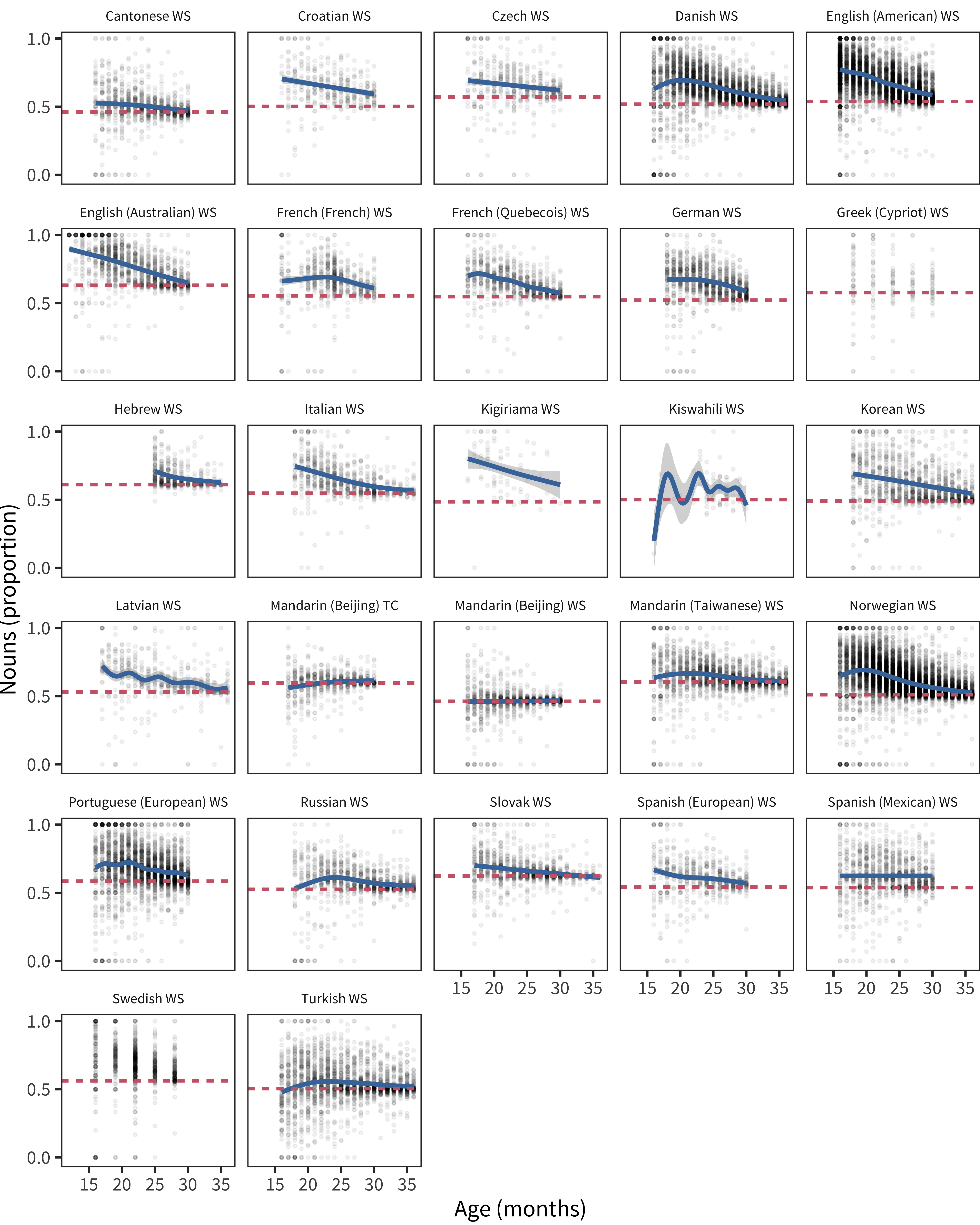
Figure 15.1: Proportion of nouns that each child produces as a function of age, with the blue curve showing a smoother fit and the red line indicating the proportion of nouns on the form.
Is a referential style associated with having a larger vocabulary? If so, then the proportion of nouns in a child’s vocabulary should be a predictor of vocabulary size, over and above age.
A simple model of this hypothesis is a generalized linear model predicting the number of CDI words a child produces as a function of age and proportion of nouns.29 The coefficients of such a model, fit to the data from each language, are shown in Figure 15.2. Age coefficients are positive, indicating more words with age. Proportion of nouns is also negative, indicating that having more nouns is related to a smaller vocabulary, controlling for age. (Confidence intervals are plotted, but are typically tiny and hence invisible.) This result appears to provide support for the opposite to the claimed relationship between the referential/expressive distinction and vocabulary size. Those children with more referential vocabularies have smaller vocabularies, controlling for age.
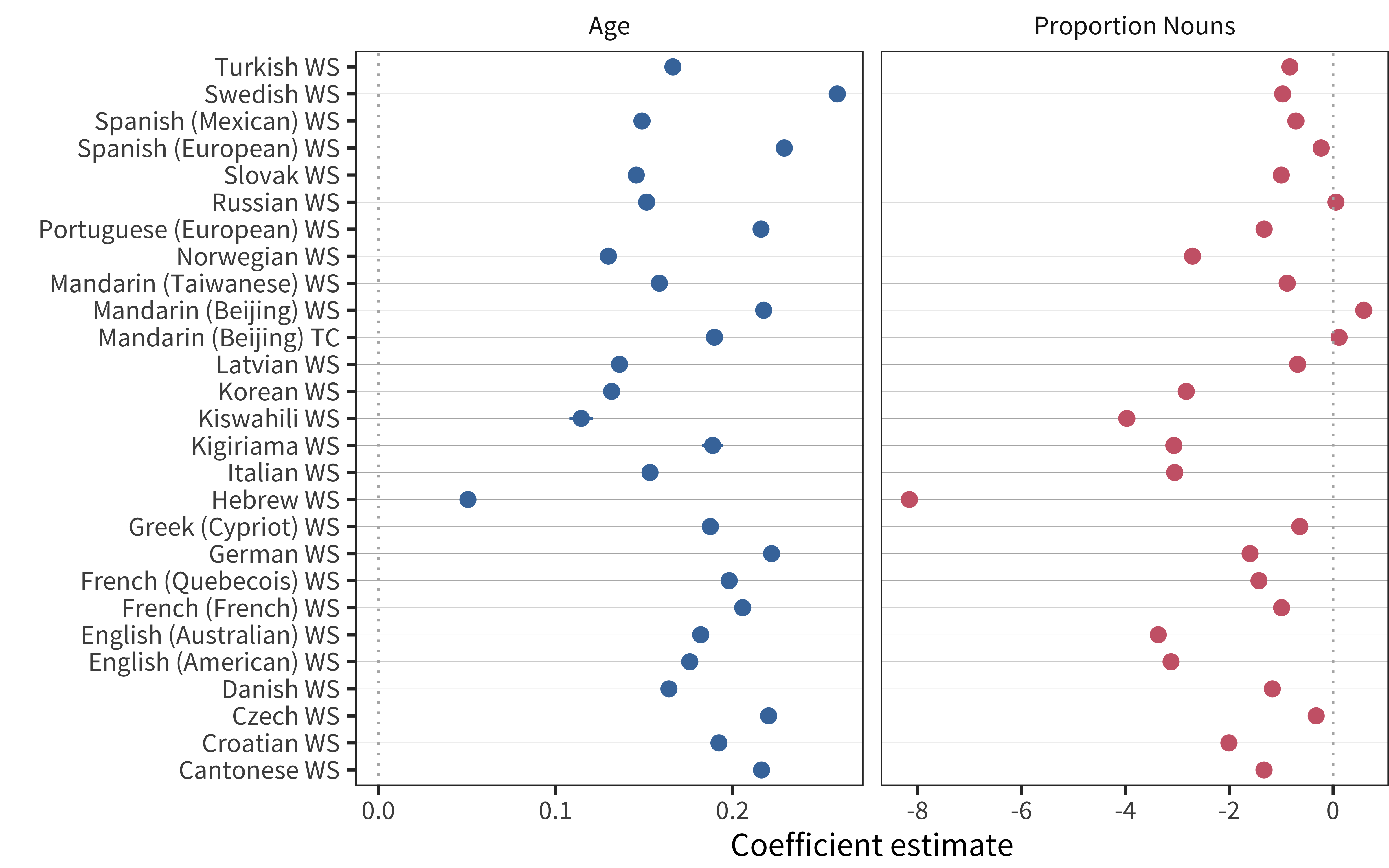
Figure 15.2: Effects of age (left) and proportion of nouns produced (right) on vocabulary size in each language.
The trouble is that these variables – age, noun bias, and total vocabulary size – have a complex relationship to one another. For a young child, having a bigger noun bias is correlated with having a bigger vocabulary (because they are on the early part of the “noun over-representation” curve shown in Chapter 11). In contrast, for an older child, having a bigger noun bias is correlated with having a smaller vocabulary because they are on the later part of the curve. Thus, the directionality of the relationship that you discover is largely determined by what part of your sample is densest.
Put another way, proportion of nouns could be predictive of vocabulary size not because children with a particular style have bigger vocabularies, but because having more nouns in your vocabulary simply indicates that the child is further along a standard progression. Put another way, perhaps all children follow the same trajectory through the noun bias. Even in this scenario, knowing the size of a child’s noun bias will tell you something about vocabulary size, without that implying that the child is following a different trajectory. This point is made in different ways by both Bates et al. (1994) and Lieven, Pine, and Barnes (1992).
15.2.2 Growth-corrected vocabulary composition
One way to circumvent this critique statistically is to measure whether a particular child has a greater-than-average, vocabulary-adjusted noun-bias. In other words, if we remove the average correlation with noun bias and vocabulary, can we still find a relation with individuals’ degree of noun bias and vocabulary size?
Figure 15.3 shows both the English noun-proportion data (plotted now by vocabulary size) and the residuals of that distribution when fit via a cubic model. The next question we can ask is how this “residualized style” relates to other variables like age, grammatical ability, and (in longitudinal data) further vocabulary growth. Note that we cannot directly compare this variable to other aspects of concurrent vocabulary size because features like, for example, number of closed class items in the vocabulary are non-independent (since the more nouns you have, by definition the fewer closed class items).
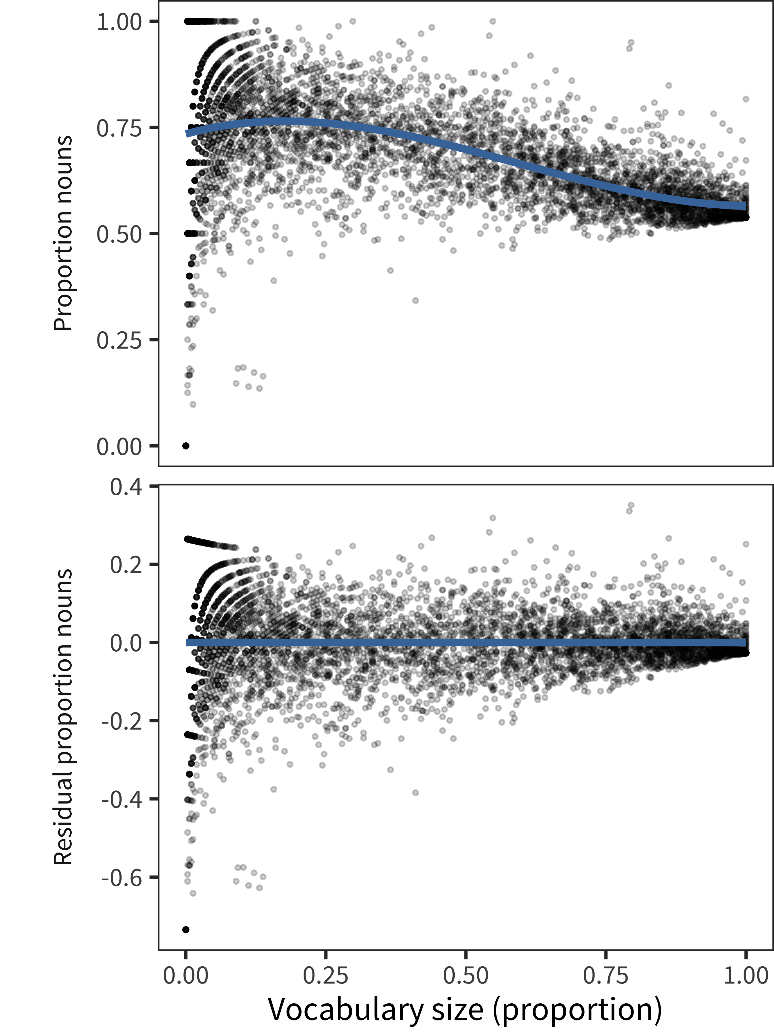
Figure 15.3: For American English data, proportion of nouns produced by each child as a function of their vocabulary size (top) and the residual proportion of nouns regressing out vocabulary size (bottom).
Our first analysis looks at the correlation between vocabulary-residualized noun bias and age. Figure 15.4 shows coefficient estimates on this analysis. Now, most age coefficients are reliably negative, suggesting that a greater residual noun bias is associated with being younger. Two of the main outliers here are from Mandarin, which, as discussed in Chapter 11, has the smallest noun bias of any of the languages in our dataset.
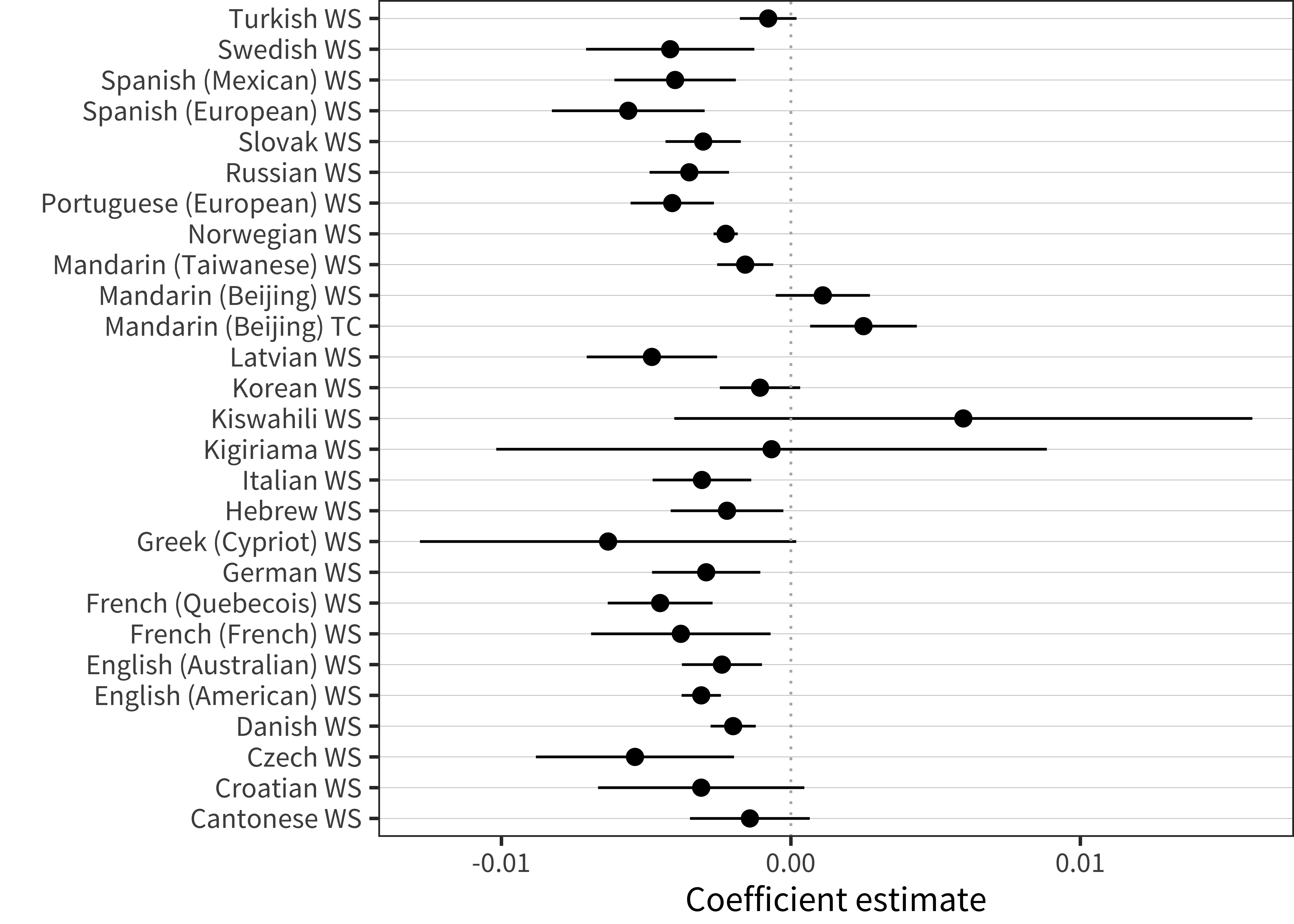
Figure 15.4: Effect of age on vocabulary-residualized noun bias in each language.
15.2.3 Vocabulary composition and grammatical ability
Lieven, Pine, and Barnes (1992) were interested in the possibility that an alternative route into combinatorial language from a referential style would be the use of construction-based generalizations. To test this hypothesis using our bias-corrected measure, we examine correlations with grammatical ability.
For grammatical complexity scores (Figure 15.5), we see that vocabulary-residualized noun bias is reliably related to grammatical complexity, as indicated by estimates that are to the left of the vertical dashed line. (Again, Mandarin is an exception). Because of the residualization procedure, this relation reflects effects that are over and above the correlations between grammar and lexicon (as reported in Chapter 13). Thus, those children with more nouns than expected for their vocabulary size produce less complex language. As seen above, they are also younger than expected.
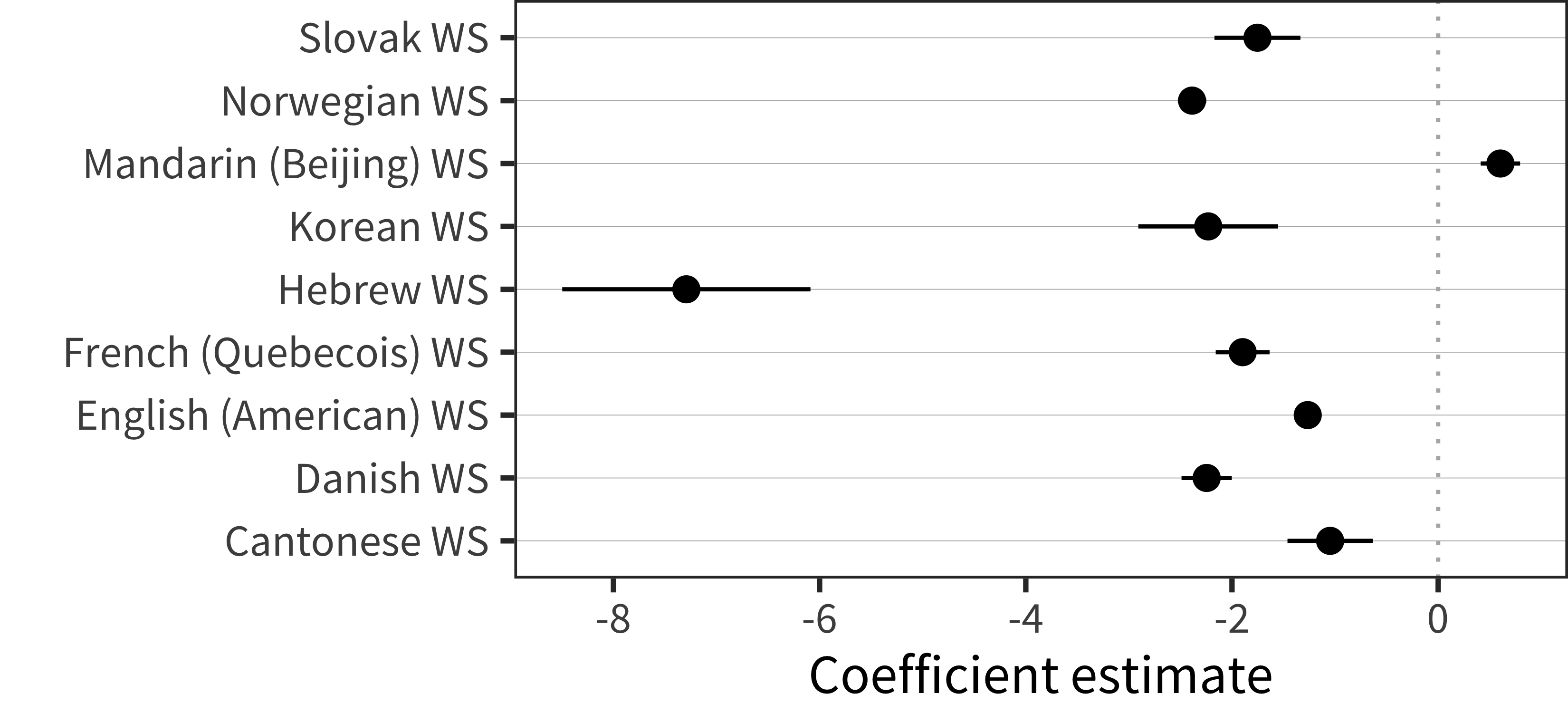
Figure 15.5: Effect of vocabulary-residualized noun bias on complexity score in each language.
We next repeat the analysis of complexity while controlling for age and total vocabulary size. The coefficients are shown in Figure 15.6. Vocabulary size, of course, has a positive relation to grammatical complexity, as does age (see Chapter 13). Even controlling for these two factors, however, we still observe a consistent negative relation between residual noun bias and complexity.
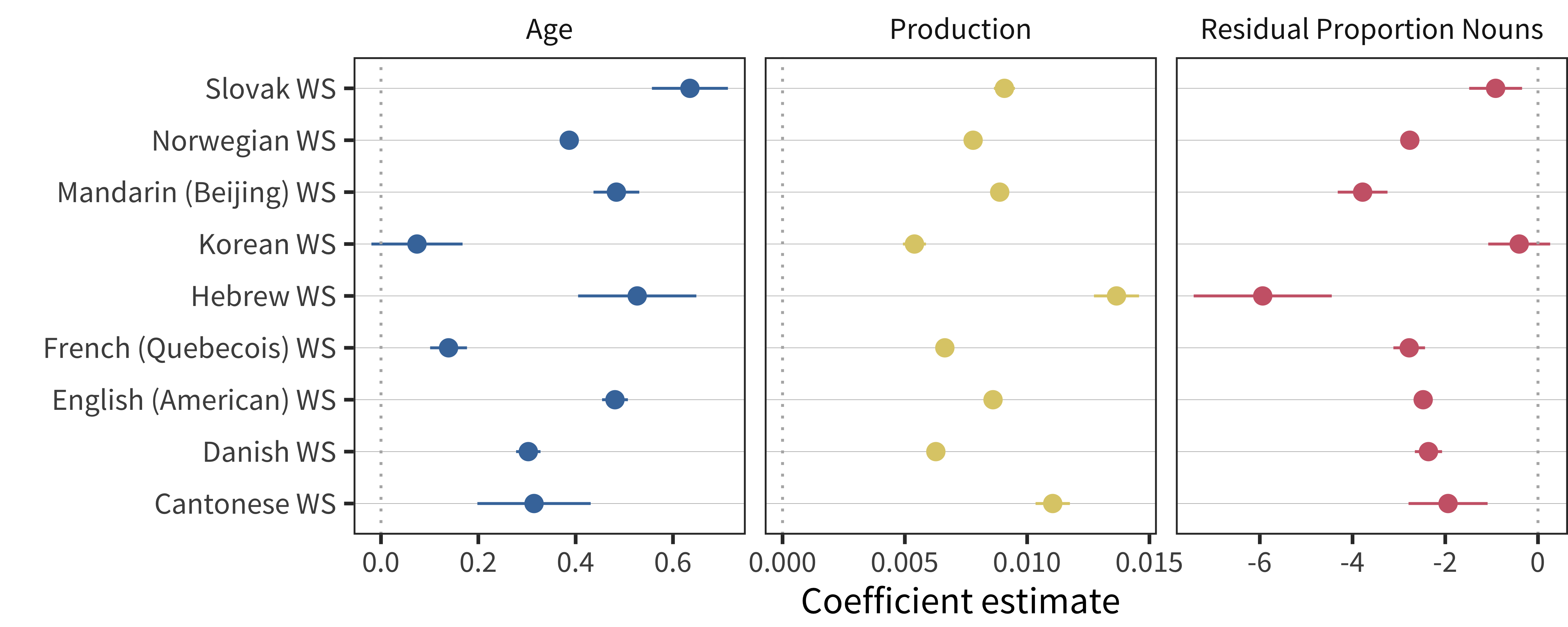
Figure 15.6: Effects of age (left), vocabulary size (middle), and vocabulary-residualized noun bias (right) on complexity score in each language.
15.2.4 Vocabulary composition differences across siblings
Nelson (1973) noted that later-born children had larger expressive vocabularies than first-born children. This observation is consistent with the confounding of vocabulary size and composition, since later-born children tend to have smaller vocabularies (see Chapter 6). But, there are other reasons to suspect that vocabulary composition could differ for children who are first vs. later born. Tomasello and Mannle (1985) observe that older siblings tend to be more directive with their younger siblings. Since more directive speech has been argued to lead to an “expressive” style, perhaps later-born children have a different vocabulary composition due to the input they receive (Tomasello and Todd 1983).30
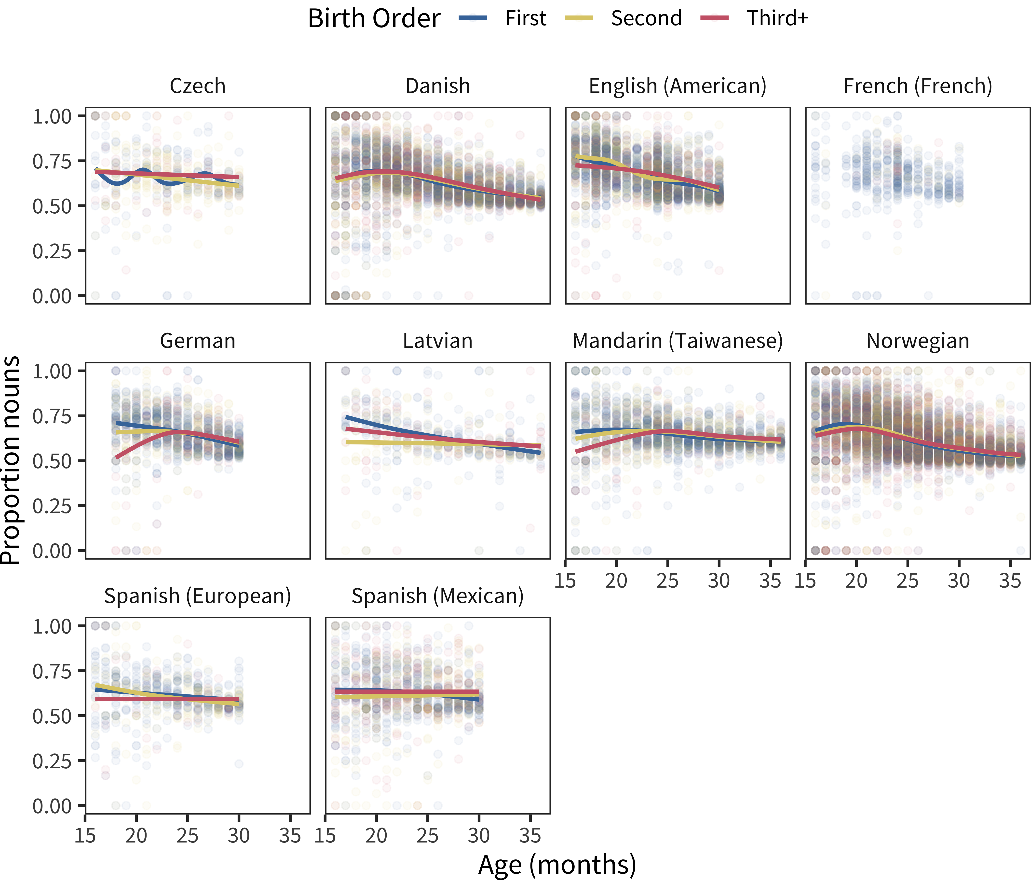
Figure 15.7: Proportion nouns in vocabulary by age, with color showing birth order.
We first examined uncorrected vocabulary composition by birth order. Figure 15.7 shows this analysis. There is a trend for young children (15–20 months) to show slightly “nounier” vocabularies – consistent with Nelson (1973)’s observation – but this trend is very small and not observed in all languages.
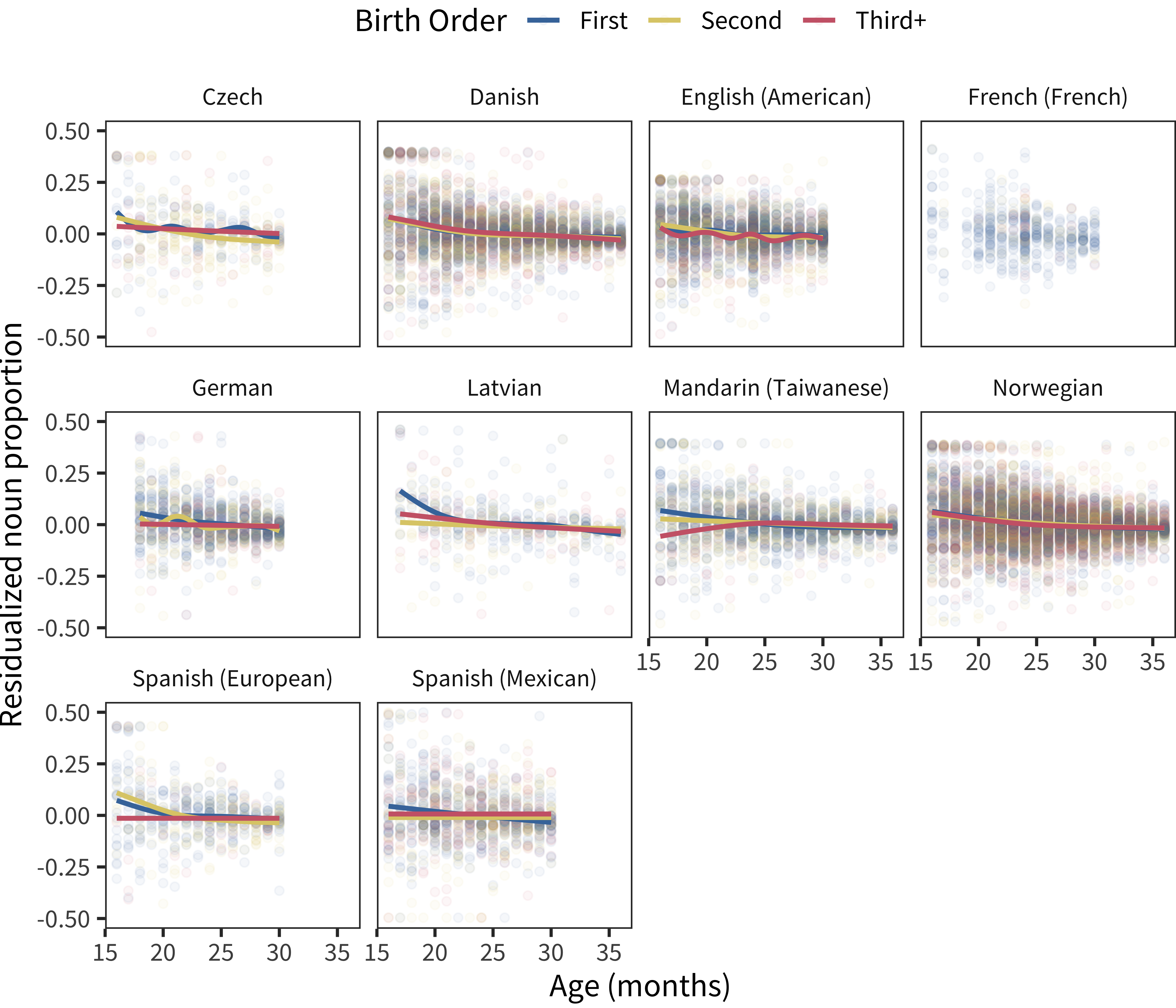
Figure 15.8: Vocabulary-residualized noun proportion by age, with color showing birth order.
Further, when we examine the trend in the residualized noun proportion, it appears even weaker and is observed in even fewer languages. This pattern is shown in Figure 15.8. Thus, we conclude that differences in vocabulary composition across birth order are likely to be small and may be, at least in part, due to faster learning by earlier-born siblings.
15.2.5 Conclusions
To summarize, we were interested in this subsection in whether we found cross-linguistic evidence for different styles of language learning, in particular, individual differences that mapped onto the referential vs. expressive distinction. Operationalizing this distinction, we asked whether children with a larger noun bias were different in their language learning trajectory than children with a smaller noun bias. The relations between overall noun bias and vocabulary are complex to interpret due to the non-linear relationships between these variables and age. To circumvent this, we examined a residualized noun bias measure that controls for total vocabulary size. Across languages, this measure was related to age and to grammatical complexity: children with relatively more nouns in their vocabulary tended to be younger and to be producing less complex speech. On the other hand, there was only limited evidence that these differences were manifest across birth orders, when controlling appropriately for overall vocabulary size (contra early speculations by Nelson 1973).
Taken together, these data provide some cross-linguistic support for the idea that children show variability beyond differences in rate of vocabulary acquisition. One dimension of variability is that, for a particular level of vocabulary size, there appear to be children who are younger, know more nouns, and combine words less (perhaps the “referential” children referred to in previous literature); other children will be older, have a more diverse vocabulary (including more predicates), and will tend to use more complex word combinations.
15.3 Spurts in vocabulary
Perhaps the most obvious aspect of early vocabulary is that it picks up speed in growth over the second year after birth. First words are hard-won, but soon children’s vocabulary acquisition appears to “explode.” This acceleration is easily visible in Figure 15.9, which shows the median productive vocabulary from 8–18 months (for American English Words & Gestures data). (We could measure the rate of learning by taking the derivative of this curve; but this rate calculation is slightly misleading for cross-sectional data and so we postpone this analysis until below). This increase in the rate of vocabulary learning has been much remarked on in the literature, as discussed above.
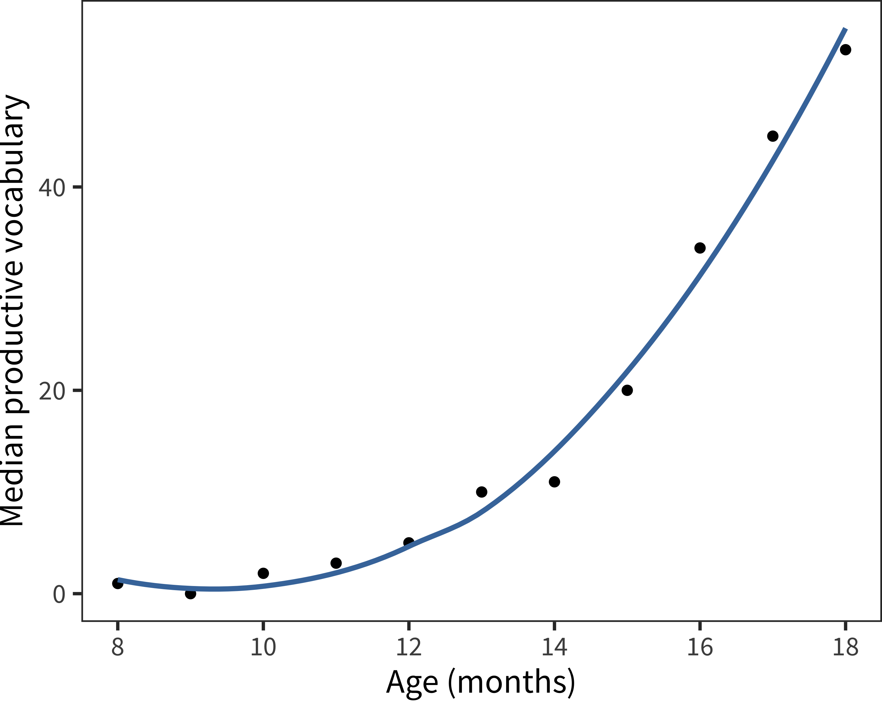
Figure 15.9: For American English data, median productive vocabulary as a function of age (curve shows smoothed fit).
Our starting point here is a study by Ganger and Brent (2004), who provide a detailed, curve-fitting analysis of the question of vocabulary “spurts.” They evaluate whether individual children’s longitudinal growth patterns are better fit by a model with constant acceleration in growth rate, or whether some children have a discontinuous “step” in terms of their growth rate.
In our view, this is a productive approach, but requires access to sufficient appropriate data that capture children’s growth rate generally. For example, using longitudinal data, we can simply examine features of rate and acceleration and how they change with time. For these analyses we focus on longitudinal production data from Norwegian and English WS and WG forms. Because we are interested in computing (potentially non-linear) changes in rate, we need four datapoints from each child as a minimum (for intercept, linear, and quadratic components). In addition, because we are interested in early changes, we set the restriction that the first time-point reported should have fewer than 50 words reported (50 words is often used as a semi-arbitrary cutoff for the onset of the vocabulary spurt; Dapretto and Bjork 2000; Ganger and Brent 2004).
The decision to exclude children with larger vocabularies at their first recorded measurement means that there is likely to be an overrepresentation of children with slower, rather than faster, rates of vocabulary growth. In particular, from the WS data, we exclude a substantial proportion of children even from the youngest groups (e.g., 22% of Norwegian 16-month-olds). So as not to bias the analysis further by including a large proportion of older, slower learners, we only include children younger than 21 months in this sample.
We now have a population of children for whom we can evaluate the rate of vocabulary growth and how it varies as a function of age. This winnowing leaves us with data from 290 children, whose growth curves are shown in Figure 15.10.
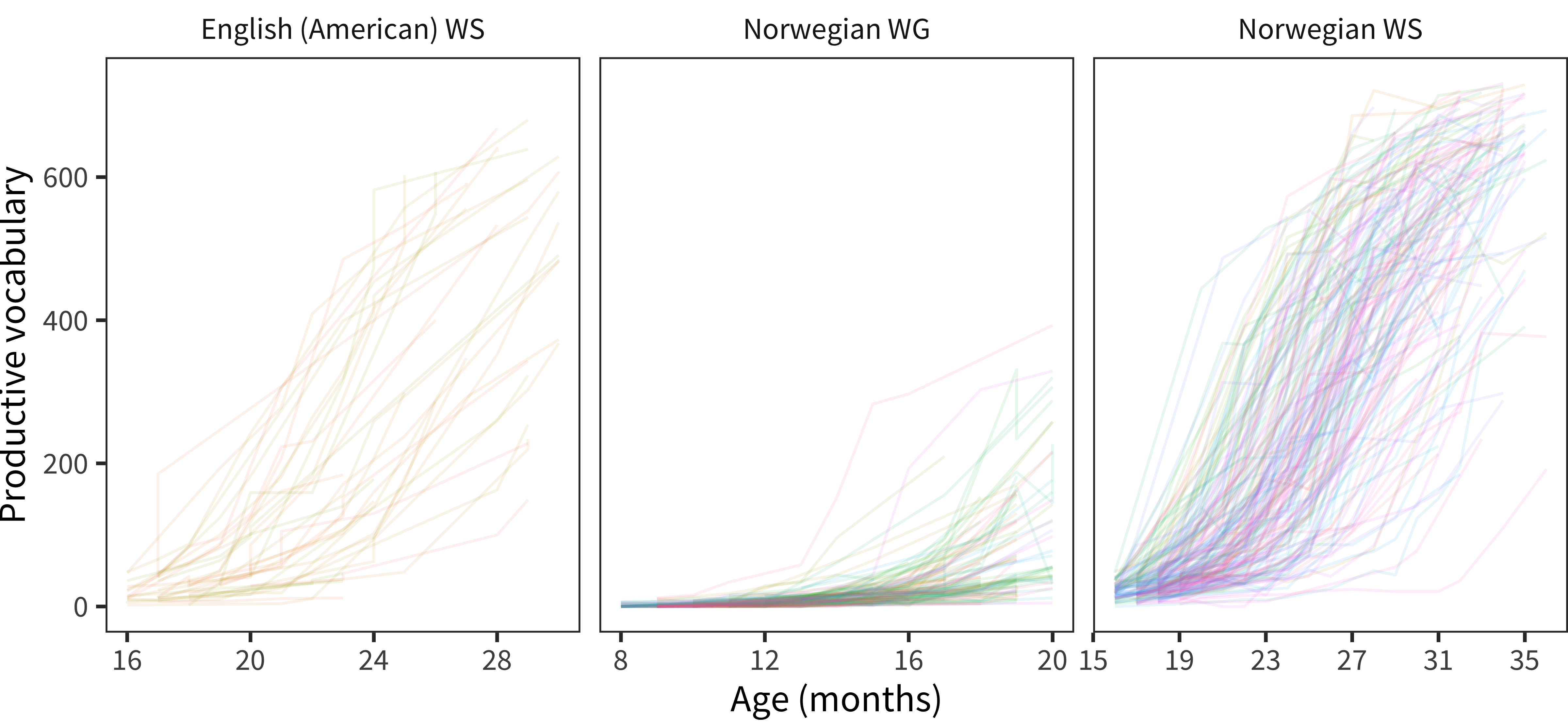
Figure 15.10: Vocabulary size as a function of age for included longitudinal administrations.
We exclude datapoints associated with large decreases in vocabulary (negative rates). Although some small negatives would be expected based on measurement error or forgetting, large negative spikes are rare and likely due to errors in the data (e.g., a partially filled form). We exclude rates of –10 words/month and below (1.3% of data).
Figure 15.11 shows children’s estimated growth rates in the period leading up to that month (number of words learned since the last longitudinal measurement divided by number of months since that measurement) plotted by total words produced in that month. There is a clear quadratic shape to this pattern, almost certainly caused by ceiling effects for children who are “running out of words” on the form.
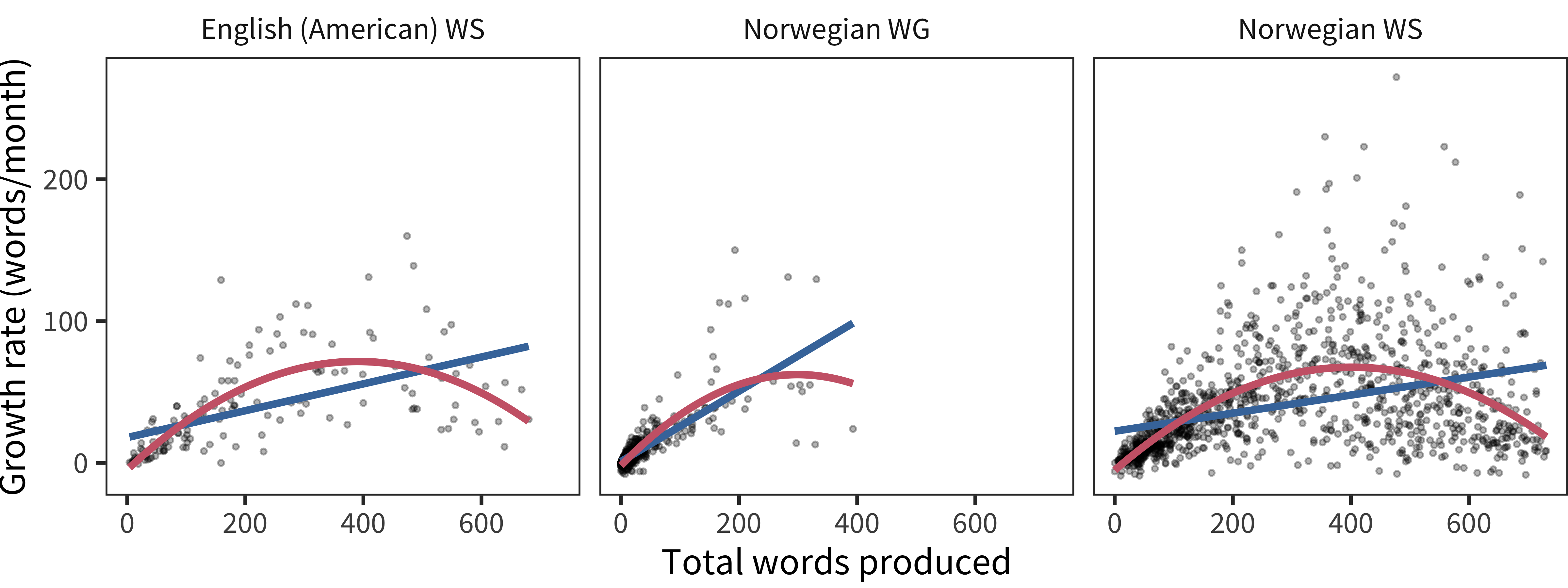
Figure 15.11: Vocabulary growth rate as a function of vocabulary size for all included longitudinal administrations (red line shows quadratic fit, blue line shows linear fit).
The definition of a vocabulary spurt, as posed by Ganger and Brent (2004), concerns the way that vocabulary growth rates may or may not increase for individual children. Clearly vocabulary growth rates increase (because vocabulary growth picks up speed generally). The question is, instead, do growth rates change smoothly, indicating constant acceleration? Or do growth rates move from one equilibrium to another (indicating a “spurt”)? Ganger and Brent (2004) proposed analyzing children’s growth rates not as a function of age, but of total vocabulary. To examine this question, we need to focus on the initial 250 words when the average rate appears to be increasing linearly (before ceiling effects are found; see red curve above), and identify children with more than 4 CDIs before this time (to ensure sufficient density). Further, we need to examine the rate trajectories of individual children. Figure 15.12 shows this analysis for a randomly sampled subset of children in our available datasets.
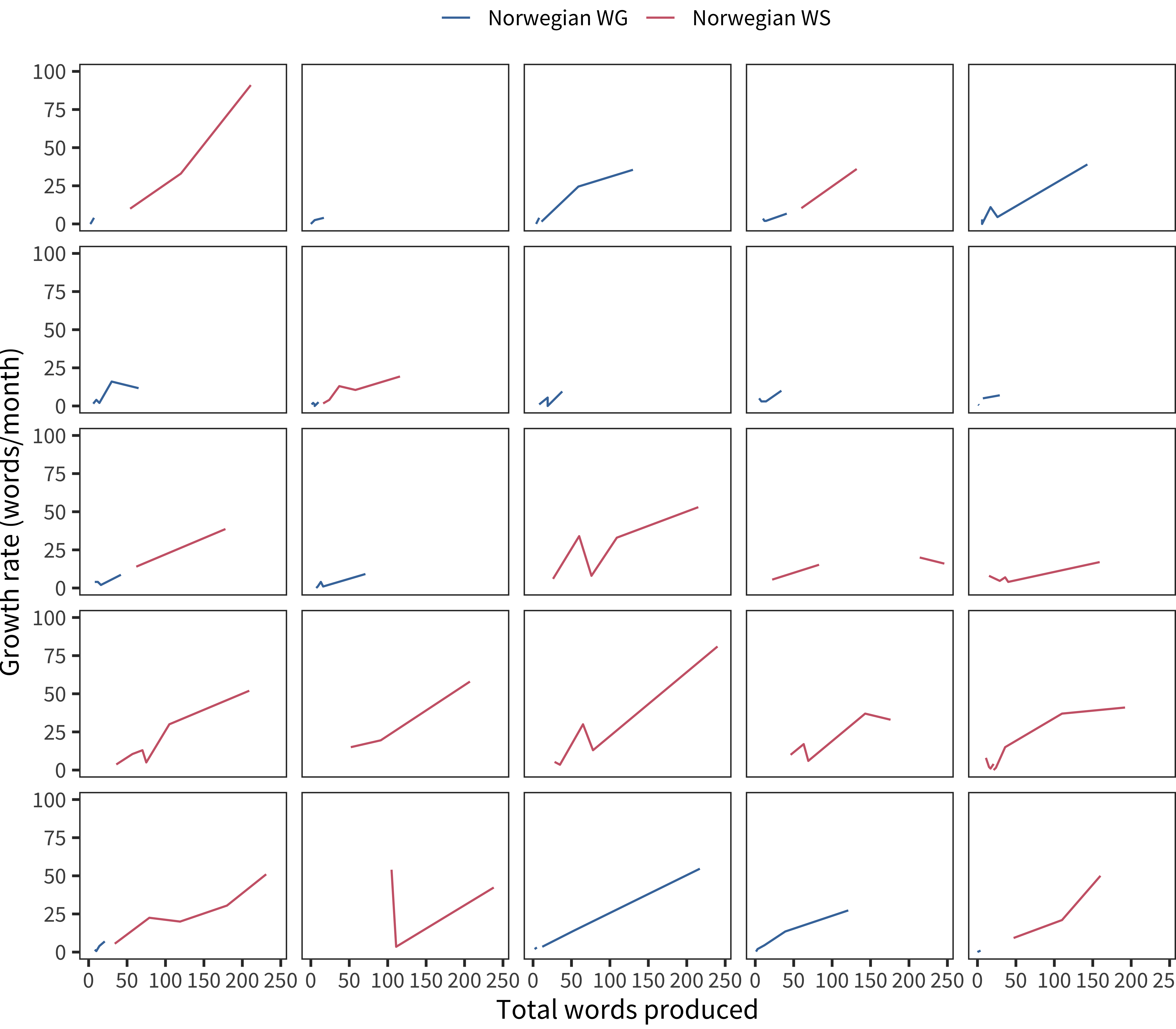
Figure 15.12: Vocabulary growth rate as a function of vocabulary size for 25 randomly sampled children.
Ganger and Brent (2004) analyzed the question of developmental spurts by fitting different curve types to the rate function in their data. They compared the likelihood ratio of quadratic and logistic rate curves for each child’s data. The quadratic curve represented the hypothesis of smooth growth in rate (smooth acceleration). In contrast, the logistic curve was of the form
\[R \sim \frac{\alpha}{1 - e^{-\beta (W - \gamma)}}\]
where \(R\) is the rate of acceleration, and it is assumed to be distributed as a function of \(\alpha\), the asymptotic rate, \(\beta\), the slope of the change between the initial and final rates, \(W\) (the total vocabulary), and \(\gamma\), the point at which the spurt occurs. This curve captures a discrete “spurt” – a movement from one equilibrium to another.
We fit these functions (as well as a simple linear function) to our data. Fitted curves for children with more than 7 datapoints are shown in Figure 15.13. The basic visual impression from these data is that, even with the longitudinal depth we have for individual children, there is substantial uncertainty in the best-fitting curve. Nevertheless, it does not appear that many children show something that looks clearly like a spurt. A few children rise quickly and then show one datapoint that levels off.
But, there is a puzzle. We can only confirm that the rate has leveled off if we have data at higher levels of production. Yet, for vocabulary sizes over 300 words, every child will level off in their rate because of the potential for ceiling effects, i.e., they have “run out of words” on the form. This example illustrates some of the difficulties in making strong inferences from data of this type.
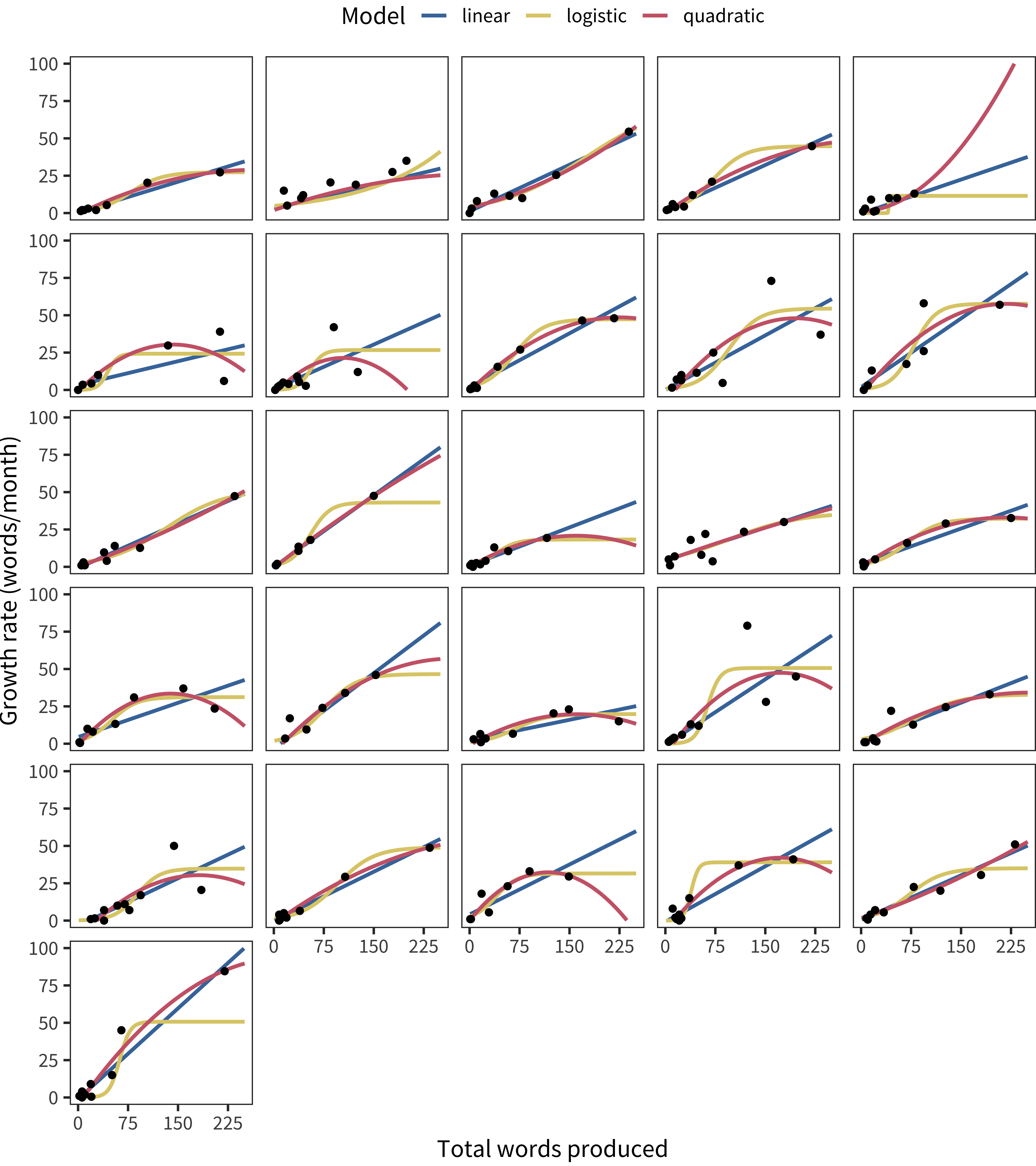
Figure 15.13: Vocabulary growth rate as a function of vocabulary size for children with more than 7 datapoints, with curves showing various model fits.
We next conducted the full model comparison analysis that Ganger and Brent (2004) conducted, over the 101 separate longitudinal records included.31 In Ganger and Brent’s analysis, they used only two models (quadratic and logistic), which had the same number of parameters. Accordingly, they compared only the likelihoods of the data under these models. In contrast, we compared a linear function with intercept at 0 (1 parameter), standard linear (2 parameters), quadratic (3 parameter), and logistic (3 parameter) curves. To make up for the difference in parameters, we computed Akaike’s Information Criterion (a measure of model goodness of fit, where smaller is better) for each model for each participant.
Table 15.1 shows the proportion of children in each dataset for which different model types fit best. Overall, children were split between models, with some children best fit by the logistic. The linear functions, which were simpler, however, fit more participants better, with the 1-parameter linear model with no intercept best fitting more children than any other.
| Instrument | Linear (no intercept) | Linear | Quadratic | Logistic |
|---|---|---|---|---|
| English (American) WS | 2 | 1 | 0 | 0 |
| Norwegian WG | 35 | 2 | 17 | 20 |
| Norwegian WS | 11 | 3 | 4 | 6 |
The 21 children (out of 101 total) with a best-fitting quadratic model are shown in Figure 15.14. Some of these children do appear to have data that are well-fit by the quadratic model. But, for many, this fit appears to be the product of a single datapoint; assuming some error, a more parsimonious model (e.g., simple linear) might do just as well. Thus, with more children but less density, our conclusion is strikingly similar to Ganger and Brent (2004): there is limited evidence for a vocabulary spurt in most children.
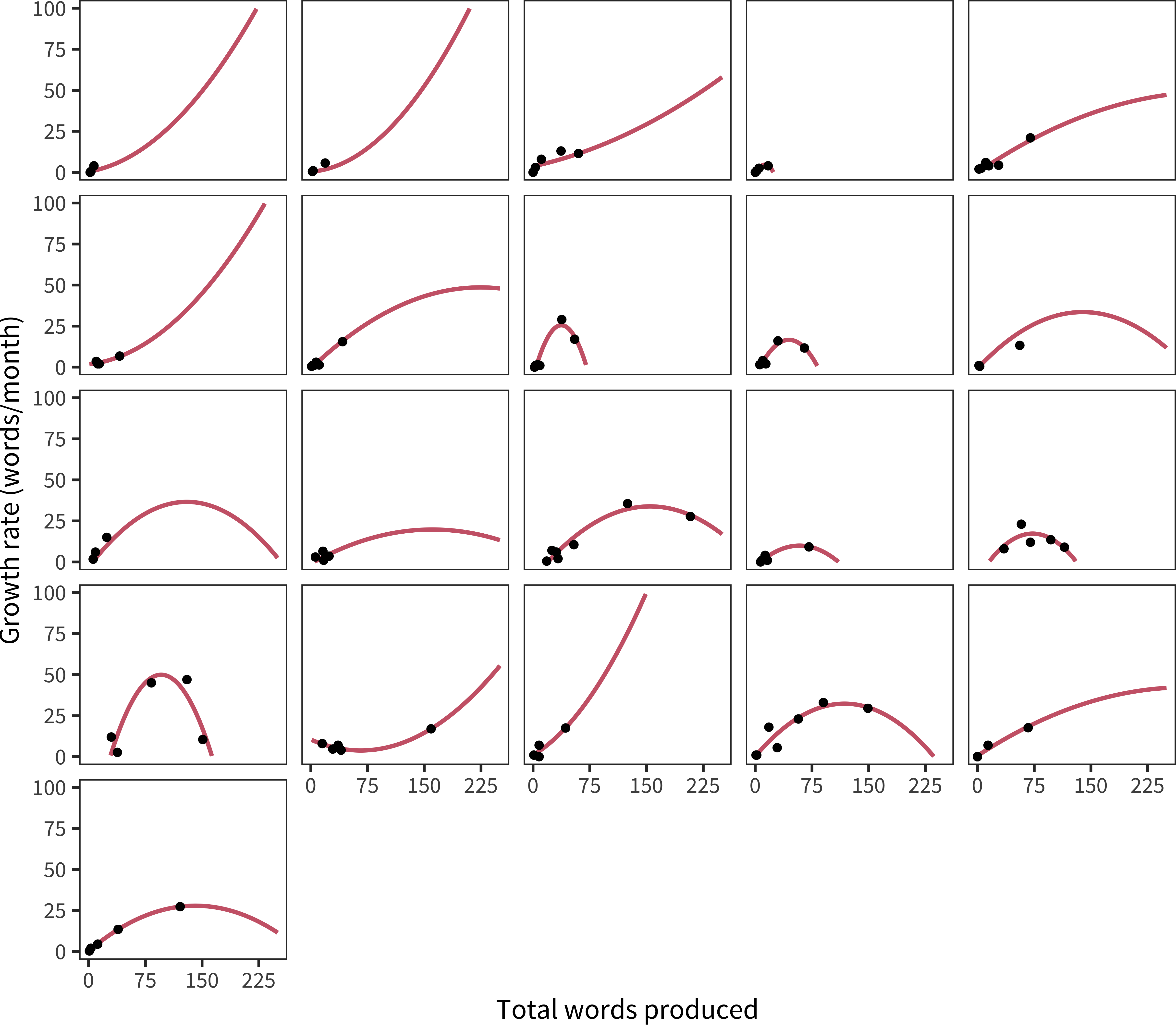
Figure 15.14: Vocabulary growth rate as a function of vocabulary size for children for whom the best fitting model is quadratic, with curves showing quadratic model fits.
To further examine this issue in a denser dataset, we used data from Roy et al. (2015)’s in-depth study of a single child. This is an ultra-dense dataset with millions of words of transcribed speech and hand-checked age-of-acquisition data for over 600 words up to the child’s second birthday. The comparable curves for this dataset are shown above. Using the same AIC method, the quadratic model fits best, but the linear model is clearly close as well.
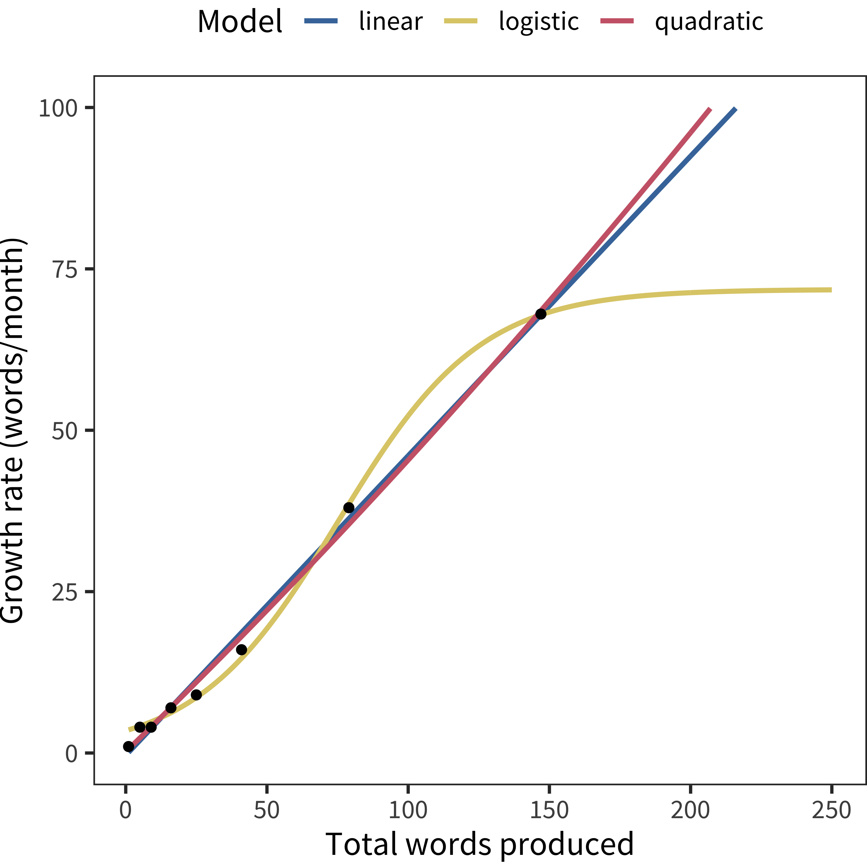
Figure 15.15: Vocabulary growth rate as a function of vocabulary size for the Roy et al. (2015) data.
Stepping back, we examined the growth rate of children’s vocabulary. To a first, group-wise approximation, children’s vocabulary growth accelerates linearly with vocabulary size during the initial period (up to around 250 words). After this point, we run into substantial measurement issues because the CDI does not contain enough words to be certain of the pattern of growth. Further, when we examined individuals’ growth, it also often appeared to be linear or quadratic; only in a minority of individuals was there any evidence for a “spurt” (a discrete change). This conclusion was tempered, however, by the difficulty of drawing conclusions without even denser longitudinal data concerning the very beginnings of language.
15.4 Variation in comprehension vs. production
Our next investigation concerns the question of how tightly comprehension and production are yoked within CDI data. Our assumption is that there is variability between children on this dimension – while some children can say a large portion of the words that they understand, others have low production scores despite appearing to understand substantial amounts. How does the ratio of production to comprehension vary across ages, and across languages?
It is important to be clear that some of the pattern in the relation between comprehension and production could be due to variation between parents in under- or over-reporting comprehension (or for that matter, production, but we assume – and Chapter 4 confirms – that production reports likely carries more signal). For example, compared to the more observable facts of word production, the variation might reflect that comprehension is a more difficult concept for parents to grasp, so there will be differences in across parents in what “comprehends” means. Some parents might be very liberal and recall a generally-understood story that included a particular word, while others might be searching for a specific anecdote that clearly illustrates comprehension of that word. We might also be detecting variation in the threshold at which parents assume that a response indicates comprehension. Nevertheless, there is evidence that children’s level of early comprehension is a useful metric for identifying possible language delays beyond production data alone. Specifically, children with only a few words who also have low comprehension scores are at increased risk for language delays compared to children with a few words who nonetheless appear to be understanding language well (e.g., Rescorla 2009).
Of course, this type of analysis can only be conducted on WG-type forms which include both comprehension and production information. We begin by investigating the American English WG data as an example.
Figure 15.16 shows individual children’s comprehension and production plotted against one another. The diagonal indicates a child who comprehends and produces exactly the same number of words. In practice, this measure is always below the diagonal because, by the design of the form, a child cannot “say but not understand” a particular word; they can only “understand” or “understand and say.”
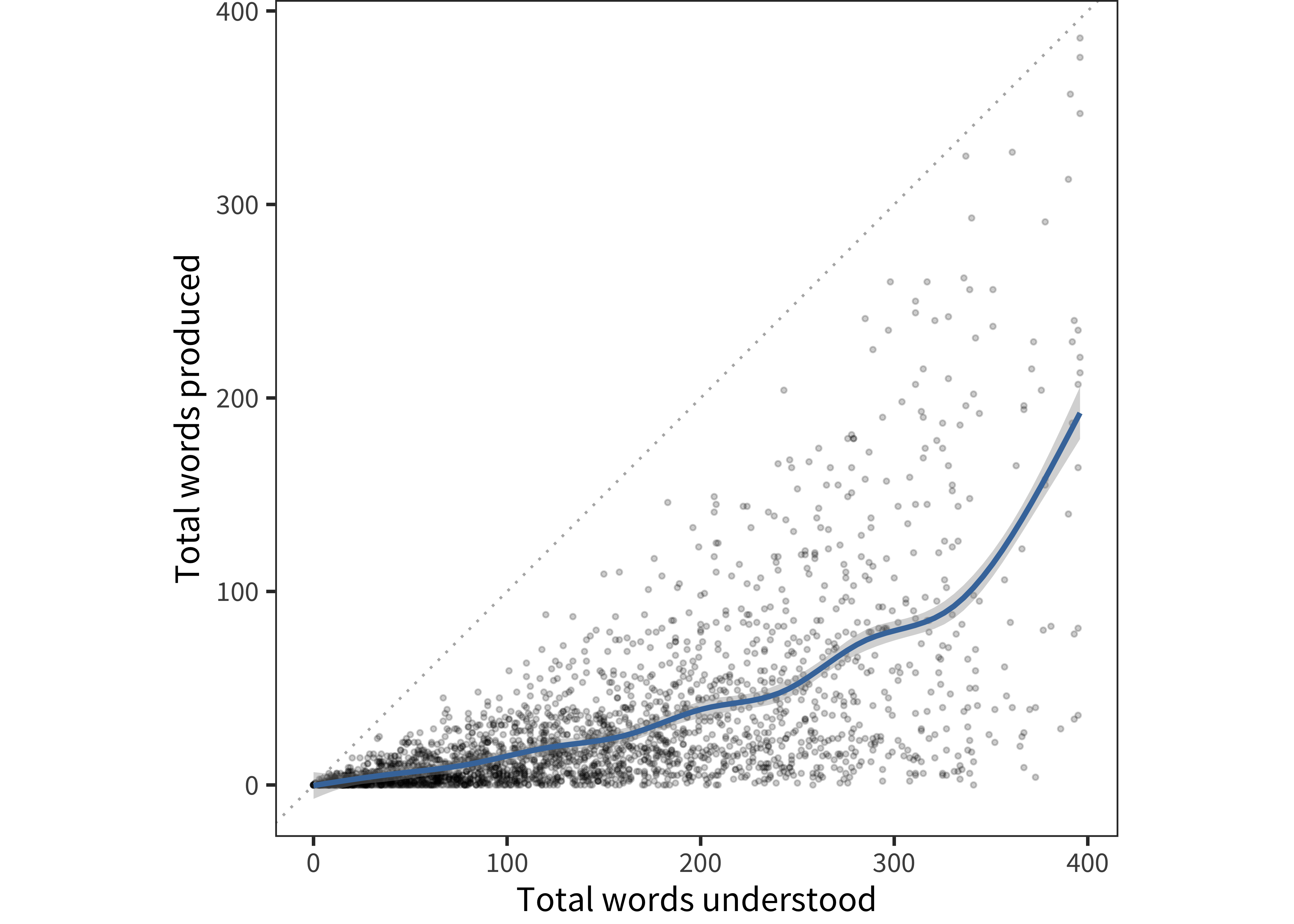
Figure 15.16: For American English data, each child’s productive vs. receptive vocabulary size.
We can convert these data into a productivity ratio:
\[\text{productivity} = \frac{\# \text{produced}}{\# \text{understood}}\] Figure 15.17 shows this ratio for all children.
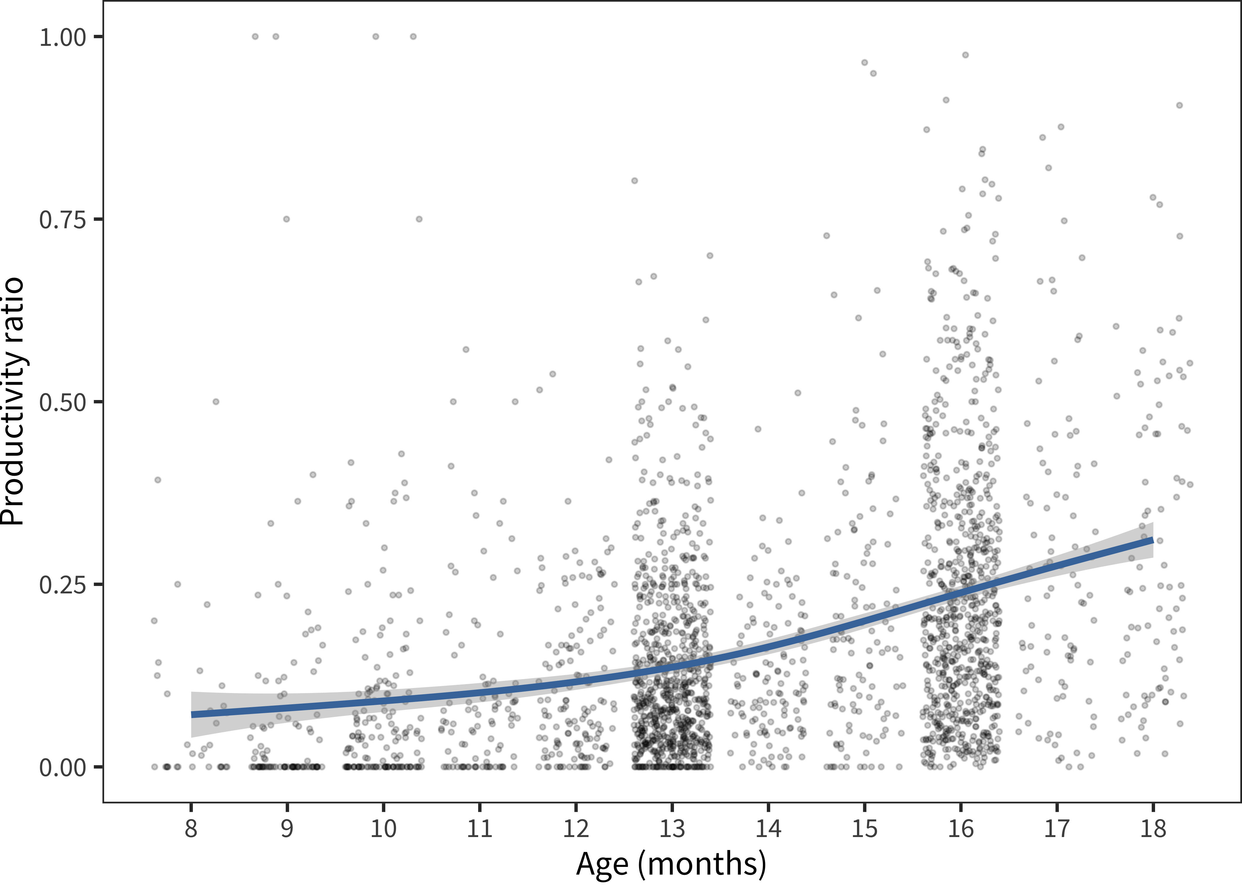
Figure 15.17: For American English data, each child’s productivity ratio as a function of age.
The resulting scatterplot is quite interpretable. It contains a few outliers at the very top of the range for very young children (whose parents report them producing and comprehending the same number of words). But, for most others, the ratio is low, increasing from about 10% to 30% by the top of the form.
Figure 15.18 plots these productivity ratios by language for an age-restricted subset between 8 and 18 months. Plots are sorted by the mean productivity ratio. While the majority of languages show the same pattern as English (an increase from around 10% to 30%), there are some outliers (Kigiriama, European French) that show a flatter slope.
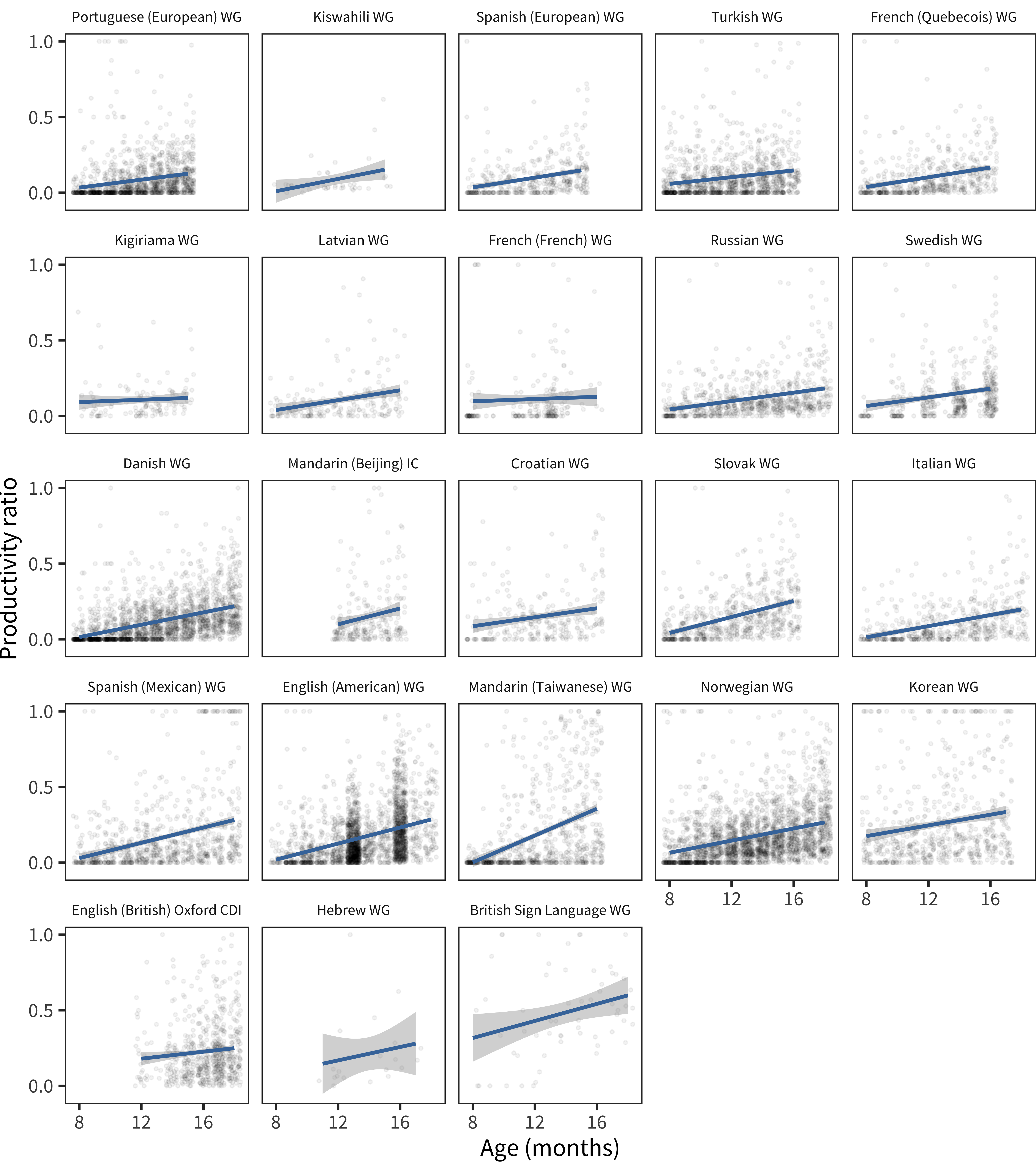
Figure 15.18: Productivity ratio as a function of age for each child in each language (lines show linear model fits).
We can see this pattern even better by plotting the best-fit lines across languages (Figure 15.19 and Figure 15.20). Nearly all of these go up with age and have similar slopes.
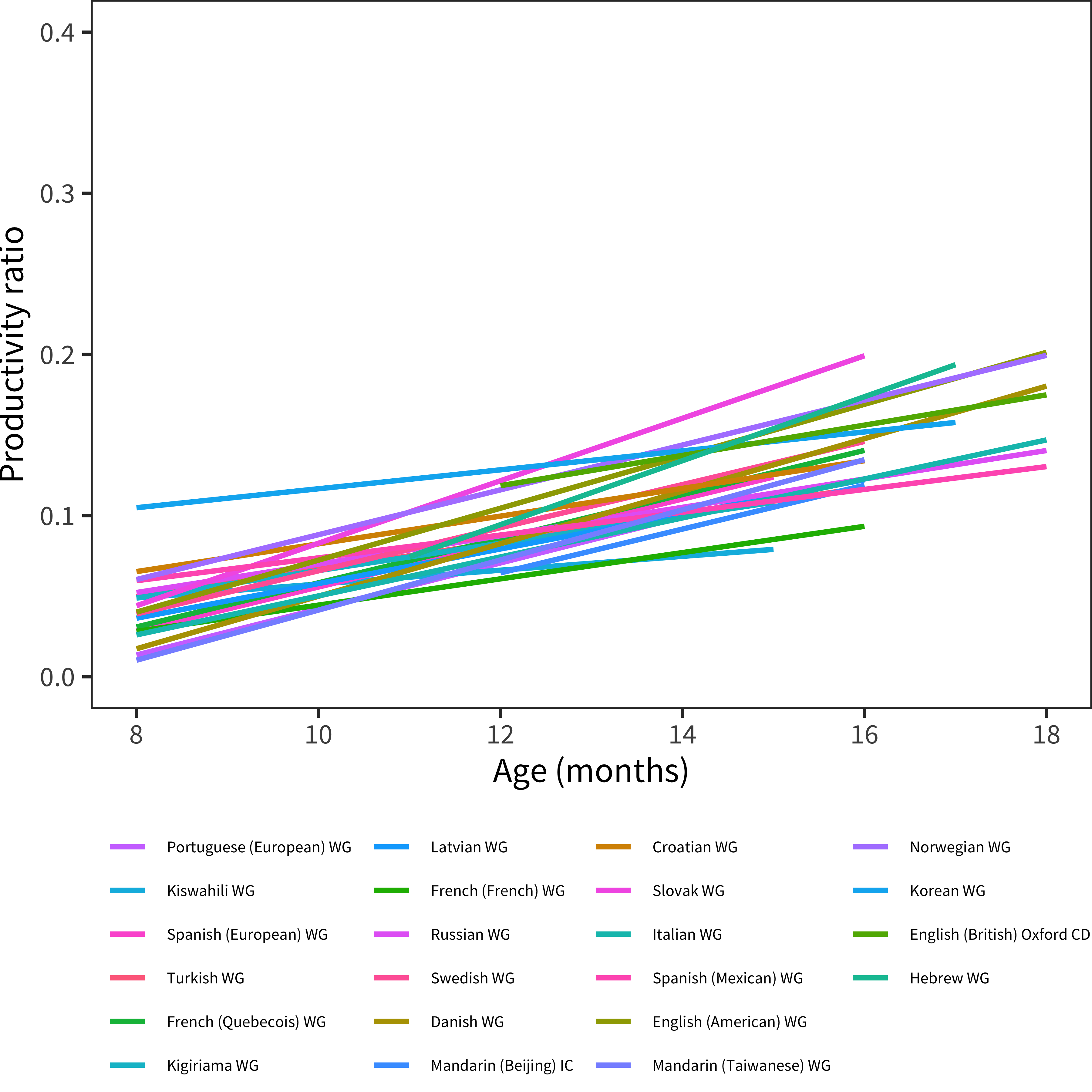
Figure 15.19: Linear model fits of productivity ratio as a function of age for each language.
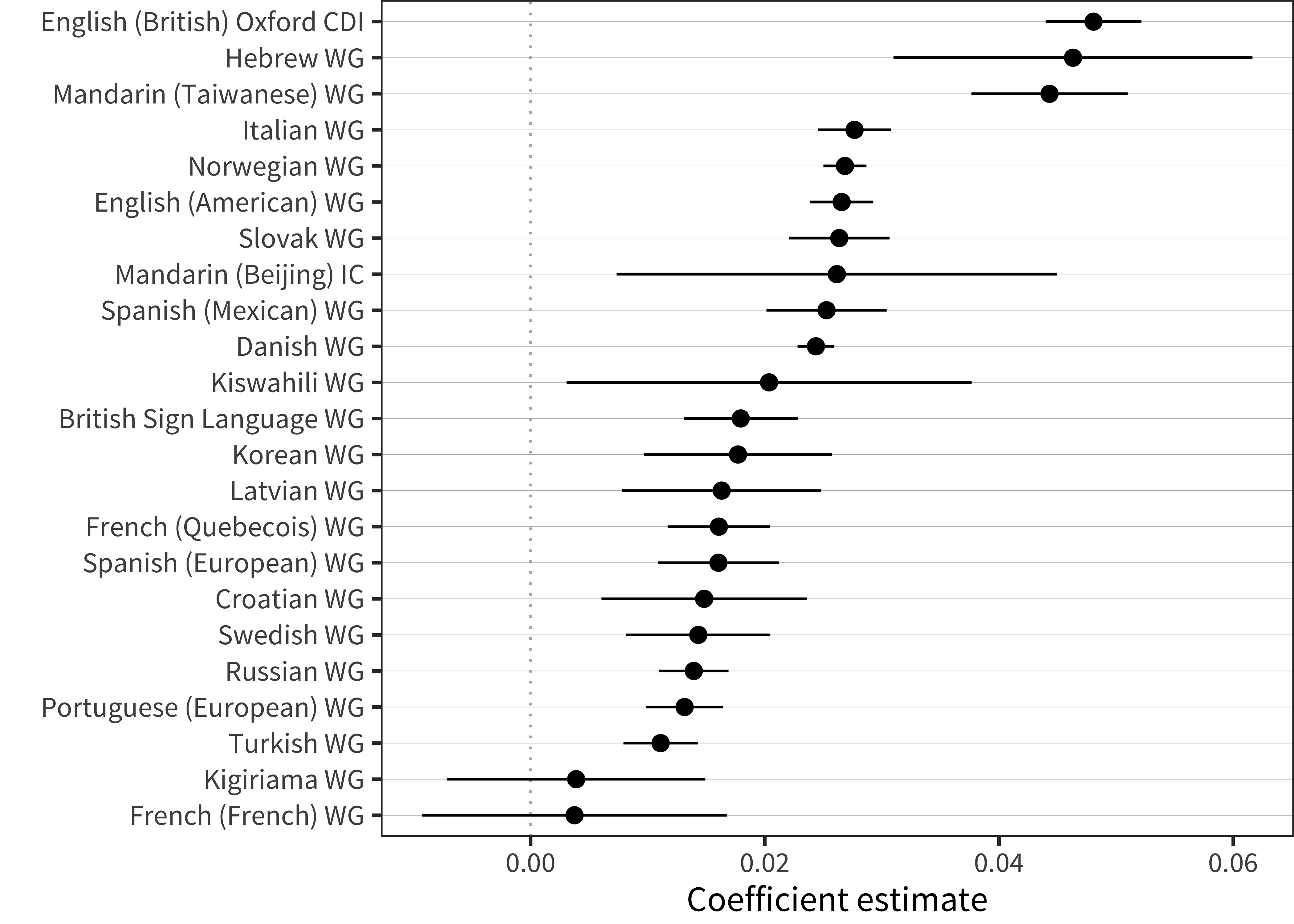
Figure 15.20: Effect of age on productivity ratio in each language (ranges indicates 95% confidence intervals).
However, in nearly every language, to one degree or another, we see some children with productivity ratios > .95. Figure 15.21 shows the proportion of children showing more than 95% productivity. A number of samples have substantial proportions of parents reporting comprehension in this way. While it is possible that these numbers represent actual children whose production is synchronized with their comprehension, a more parsimonious explanation is that there are local variations in administration, leading to some fraction of parents who are not completing the form properly. In particular, it does not appear that these “no comprehension without production” children are the tail of a shifted distribution of productivity ratios; instead, they appear to be due to a separate small population. Yet, despite that, they appear to have an outsized effect on our estimates of the development of productivity ratios across languages.
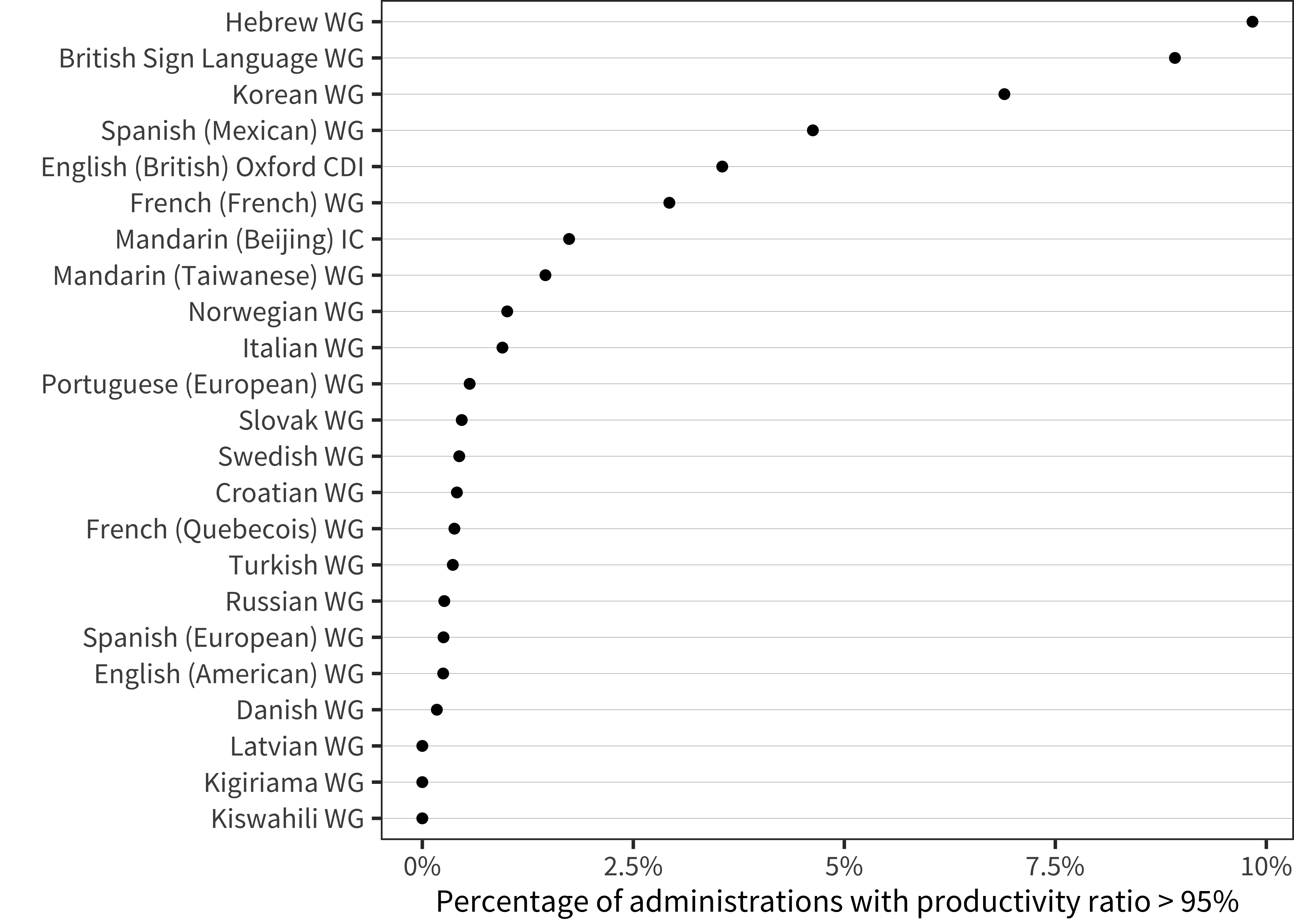
Figure 15.21: Percentage of administrations in each language for which the productivity ratio is greater than 95%.
In sum, although the relationship between production and comprehension is a fascinating locus for individual differences, we may not be able to measure this relationship effectively using cross-linguistic comprehension data. Further, these analyses underscore the importance of developing instructions for parents that more effectively convey the concept of what it means for a child to “understand” a word. Outside of these concerns, while there very well may be reliable variation in the comprehension-production ratio across children, we unfortunately do not have access to independent signals that could validate this quantity.
15.5 Discussion
In this chapter, we have explored three classic indices of individual variation in children’s “style” of learning, that is, variation in how children approach the task of language learning. Compared to differences in rate/timing of learning, stylistic differences have been proposed to be a stronger test of the proposal that language acquisition is a constructed process. Only a few studies to date have had the power and scope to explore the extent of these differences cross-linguistically.
We can summarize the conclusions from our various sub-analyses. First, we were not able to substantiate differences between individuals in production/comprehension differences. It is tricky to use comprehension data to estimate variability between individuals in how much they produce vs. comprehend, due to likely differences across sites (and thus, across languages) in the uptake of instructions regarding what “comprehension” means. In contrast, we did see support for the traditional referential vs. expressive distinction from cross-linguistic analysis. We found that, at a given level of vocabulary size, some children tend to be younger, use more nouns at a given vocabulary size, and combine less; others tend to be older, know more predicates, and combine words more. Finally, confirming previous work by Ganger and Brent (2004), we found no evidence supporting the notion that a “vocabulary spurt” occurs universally for all children. Instead, we found that, while vocabulary growth accelerates, that acceleration is approximately linear for the first 250 words, and hence a “vocabulary spurt” is reliably observed in only a small portion of children.
These analyses do confirm the existence of stable individual variation in language learning “style.” Our work also highlights the methodological difficulty of this enterprise, however; despite the tremendous amount of data we have access to, our analyses still suffer from the limitations of the parent-report format of the CDI. It is often difficult to tell whether we are measuring children’s style of learning or parents’ style of reporting. Overcoming this limitation would require non-parent report measures with equivalent domain breadth, psychometric stability, and sample diversity to the CDI. At present to our knowledge, no publicly available datasets of this type exist.
Further, we want to highlight one potential source of some of the variation we observed: differences in children’s speech-motor ability. Children’s ability to produce complex phonological forms (e.g., Dromi 1987; Clark 2016) and complex phrases (e.g., Demuth and Tremblay 2008) both change substantially during the developmental period we are examining. Although we have not had much to say here about these changes – due to the emphasis of the CDI on content, rather than form – variability in this developmental pattern could be an important driver of the changes we observed here. Of course, speech-motor variability could be one source of variability in production-comprehension differences: children who have a harder time producing distinct word forms might nonetheless have a large vocabulary. In addition, speech-motor variability might also play a role in children’s position on the referential-expresssive continuum. Children with slower speech-motor development could be those children who are relatively more expressive in style. They would be older for their relative vocabulary size due to their delays, and due to their greater language experience might also be better at combining words. Testing this sort of speculation would be a worthy goal for a data-collection effort aimed at characterizing variability in children’s naturalistic speech across a large, consistent sample.
Caught up in this issue is the question of whether there is a route into language via the memorization of “frozen phrases.” This is an independent theoretical question that is difficult to address with CDI data as it is a question about the repetitive use of chunks of language in production. One observation is that, due to evidence of early verb generalization (e.g., Gertner, Fisher, and Eisengart 2006), the original discussion about limited generalization in children’s early syntax has been somewhat subsumed into a discussion about differences between general comprehension and conservative production.↩︎
We omit interactions from most of the models below for interpretability; including interactions leads to unstable coefficient estimates.↩︎
Technically, the observation that directive speech leads to expressive style could also be due to confounding of amount of speech; more directive parents also tend to be those who talk to children less (e.g., Hart and Risley 1995).↩︎
This number consolidates data between WG and WS forms when a child has both, to maximize our use of the available longitudinal data.↩︎